Week - 2 - Explicit and Implicit Analysis
AIM:- To study the Explicit and Implicit scheme of analysis so that we can use them to solve our engineering problems in LS-Dyna.
Also, our aim is to solve, `F(u)=u^3+9u^2+4u` by both explicit and implicit methods (with tolerence value of 0.001).
EXPLANATION:-
EXPLICIT ANALYSIS:-
LS-Dyna works mostly with explicit analysis. LS-Dyna is known for its work mainly with explicit analysis.
Explicit method is a function of time. This method needs function of time, velocity, acceleration, mass & damping.
Time increment in explicit analysis is very short. Time step is limited by the size of the numerical stability. If time step is very large, there will be significant numerical errors. Hence, explicit method works in timestep increments which means that the displacements are calculated as the time proceeds.
Explicit method is suitable for the higher dynamic analysis, such as high velocity impact. Also, LS-Dyna is known for its high dynamic problem solving features. Hence, explicit method is mostly used in LS-Dyna.
IMPLICIT ANALYSIS:-
Major difference between explicit & implicit analysis is that implicit analysis is not a function of time. So, velocities & acceleration, which are time derivatives of displacement, become zero.
Newton-Raphson iterations are usd to enforce equilibrium before moving to next step while solving. Solution is obtained in several steps and the solution of currents step is based on the solution from the previous step. Very large deformation problems such as crash analysis can result in millions of degrees of freedom, thus increasing the size of stiffness matrix. Larger stiffness matrix leads to larger computational time & cost.
Hence, implicit method is mostly not used to solve dynamic problems. Explicit method is preferred in dynamic problems. Implicit methods are more often used in softwares such as Ansys, Abaqus etc.
Explicit Method for solving given problem in this challenge:-
`f(u)=u^3+9u^2+4u` ------ equation (1)
Differentiating force with respect to displacement gives stiffness (k) of the bar. (Since F=kx)
Stiffness `k(u)= (df)/(du)=3u^3+18u+4` ------ equation (2)
Variables are as follows:-
- U = Displacement
- F = External Force
- k = Stiffness
- `Deltau` = Incremental Displacement
- `DeltaF` = Incremental Externally Applied Force
STEP 1 :-
Taking `u underset0`= 0
`DeltaF=1`
From equation 2, we get
`Deltau underset1`= `(DeltaF)/(3times0^2+18times0+4)`
`Deltau underset1`= 0.25
`u underset1`= `u underset0`+`Deltau underset1`= 0.25
STEP 2 :-
Taking `u underset1`= 0.25
`DeltaF=1`
From equation 2, we get
`Deltau underset2`= `(DeltaF)/(3times0.25^2+18times0.25+4)`
`Deltau underset2`= 0.115
`u underset2`=`u underset1`+`Deltau underset2`= 0.365
STEP 3 :-
Taking `u underset2`= 0.365
`DeltaF =1`
From equation 2, we get
`Deltau underset2`=`(DeltaF)/(3times0.365^2+18times0.365+4)`
`Deltau underset2`= 0.0911
`u underset2`= `u underset1`+ `Deltau underset2`= 0.46
Determination of force equilibrium:-
F(external) = `DeltaF+DeltaF+DeltaF = 1+1+1=3`
F(internal) = `u^3+9u^2+4u`
F(internal) = `(0.46^3+9times0.46^2+4times0.46)`
F(internal) = 3.841
`therefore`F(external) `!=`F(internal)
Hence, it is evident that external and internal forces are not in equilibrium.
Tabular Column For Explicit Analysis:-
| STEPS | `DeltaF` | `Deltau` | `u` | F(external) | F(internal) | [F(internal)-F(external)]=R |
| 1 |
1 |
0.25 | 0.25 | 1 | 1.578 | 0.578 |
| 2 | 1 | 0.11 | 0.37 | 2 | 2.708 | 0.708 |
| 3 | 1 | 0.09 | 0.46 | 3 | 3.841 | 0.841 |
Graph of Force v/s Displacement for Explicit Analysis:-
Implicit Method for solving given problem in this challenge:-
Note:- To minimize the residual, Newton-Raphson iterations are used.
Expanding residual as a Taylor's series about the current displacement gives:-
`R^(j+1)=R^j (u^j)+(dR(u^j))/(du)deltau^(j+1)+....=R^j+k(u^j)deltau^(j+1)+....`
by neglecting higher order terms in the series,
`deltau^(j+1)=-[k(u^j)]^-1R^j`; is obtained.
STEP 1:-
Taking `u underset0`= 0
`DeltaF=1`
From equation 2, we get
`Deltau underset1`=`(DeltaF)/(3times0^2+18times0+4)`
`Deltau underset1`= 0.25
`u underset1`=`u underset0`+`Deltau underset1`= 0.25
F(external) = `DeltaF=1`
F(internal) = `u^3+9u^2+4u`
F(internal) = `0.25^3+9times0.25^2+4times0.25=1.57`
R(`u underset1`) = F(internal) - F(external) = 0.57
`|\|R^(0)|\|>10^-2` `therefore`Newton-Raphson iterations are necessary.
Calculating correction `u underset1`=`u^0`
`deltau^1=-[k(u^0)]^-1timesR^0=-(3times0.25^2+18times0.25)-1times0.578=-0.0665`
Updating value of `u^1=u^0+deltau^1=0.184`
Checking again,
F(external) = `DeltaF=1`
F(internal) = `u^3+9u^2+4u=0.184^3+9times0.184^2+4times0.184=1.043`
R(`u underset1`) = F(internal) - F(external) = 0.043
`0.043>10^-2`; Hence, another iteration is needed here.
Calculating Correction `u underset 1`= `u^1`
`deltau^2=-[k(u^1)]^-1timesR^1=-(3times0.0665^2=18times0.0665)-1times0.043=-0.0714`
Updating Value of `u^2=u^0+deltau^2=0.1786`
Checking again,
F(external) = `DeltaF=1`
F(internal) = `u^3+9u^2+4u=0.1786^3+9times0.1786^2+4times0.1786=1.0071`
R(`u underset1`) = F(internal) - F(external) = 0.0071
`0.0071 < 10^-2`; further iterations are not needed.
`u underset1`= 0.1784
STEP 2 :-
`u underset1`= 0.1784
k(`u underset1`) = `3times0.1784^2+18times0.1784+4=7.3068`
`DeltaF=1`
`Deltau underset2`= `(1)/7.306813=0.1368`
`u underset2`=`u underset1`+ `Deltau underset2`= `0.1784+0.1368=0.3152`
F(external) = `DeltaF+DeltaF = 1+1=2`
F(internal) = `(u2)^3+99u2)^2+4u2`
F(internal) = `(0.3152)^3+9(0.3152)^2+4(0.3152)=2.1868`
R = F(internal) - F(external) = 2.1868-2 = 0.1868
`|\|R^0|\|>10^-2`;
`therefore`Newton-Raphson iterations are necessary.
So, k(`u underset2`) = `3u1^2+18u1+4`
`3times0.3152^2+18times0.3152+4=9.9727`
So, Calculating Correction,
`u underset1``=u1^0`
`deltau^1=-[k(u^0)]^-1R^0`
`deltau^1=-[9.9727]^-1times0.1868`
`deltau^1=0.01873`
Updating Value;
`u2^1=u2^0+deltau^1`
`u2^1=0.3152+(-0.01873)`
`u2^1=0.2965`
Checking Again;
`F undersetE`= `DeltaF+DeltaF=1+1=2`
`F undersetI`= `(u2^1)^3+9(u2^1)^2+4u2^1`
`F undersetI`= `0.2965^3+9times0.2965^2+4times0.2965=2.00356`
Now, `R^1=``F undersetI`-`FundersetE`
`R^1=2.00356-2=0.00356`
`|\|R^0|\|<10^-2`
So, further iterations are not needed.
`thereforeu underset2``=0.2965`
STEP 3 :-
`u underset2``= 0.2965`
k(`u underset2`) = `3 times0.2965^2+18times0.2965+4=9.60133`
`DeltaF=1`
`Deltau underset3``=(1)/9.6031=0.1041`
`u underset3``= u underset2``+ Deltau underset3`
`u underset3``= 0.2965+0.1041=0.4006`
`F undersetE``= DeltaF+DeltaF+DeltaF=1+1+1=3`
`F undersetI``=(u3)^3+9(u3)^2+4u3`
`F undersetI``=0.4006^3+9times0.4006^2+4times0.4006=3.1119`
`R=F undersetI``-F undersetE``=3.1119-3=0.1119`
`|\|R^0|\|>10^-2`
Hence, Newton-Raphson iterations are necessary.
So, k(`u underset3`)`=3timesu3^2+18timesu underset3``+4`
`=3times0.4006^2+18times0.4006+4=11.6938`
So, Calculating new total correction to `u2=u2^0`
`deltau^2=-[k(u3^0)]^-1R^0`
`deltau^2=-[11.6938]^-1times0.11194`
`deltau^2=-0.0095`
Now, Updating the value;
`u3^1=u3^0+deltau^2`
`=0.4006+(-0.0095)`
`u3^1=0.3911`
Now, Checking Residuals,
`F undersetE``=DeltaF+DeltaF+DeltaF=1+1+1=3`
`F undersetI`=`=(u3^1)^3+9(u3^1)^2+4(u3^1)`
`F undersetI``=0.3911^3+9times0.3911^2+4times0.3911=3.0009`
Now, `R^1=F undersetI``-F undersetE``=3.0009-3=0.003563`
`|\|R^0|\|<10^-2`
So, Newton-Raphson iterations are not necessary.
So, Final value is `u2=u3^1=0.3911`
Tabular Column For Implicit Analysis:-
| STEPS | `DeltaF` | `Deltau` | `u` | F(external) | F(internal) | [F(internal)-F(external)]=R |
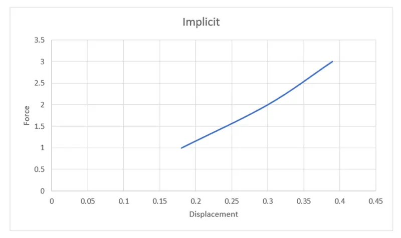
| 1 | 1 | 0.25 | 0.18 | 1 | 1.007 | 0.0071 |
| 2 | 1 | 0.1374 | 0.30 | 2 | 2.004 | 0.0042 |
| 3 | 1 | 0.1041 | 0.39 | 3 | 3.000 | 0.0008 |
Here, `F undersetE``= F undersetI`
Hence, it is evident that the external forces & internal forces are in equilibrium.
Graph of Force v/s Displacement for Implicit Analysis:-
Exact Solution:-
`f(1)=u^3+9u^2+4u`
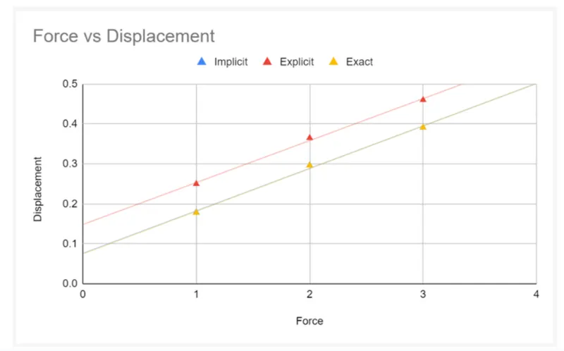
`u underset1``=0.17762`
`f(2)=u^3+9u^2+4u`
`u underset1``=0.29616`
`f(3)=u^3+9u^2+4u`
`u underset1``=0.39103`
Comparison graph of Force v/s Displacement between Implicit & Explicit Analysis:- (Exact Calculations)
CONCLUSION:-
Initial increment due to incremental load, advances the solution forward. If implicit analysis is used, Newton-Raphson iterations are used to make corrections to the displacement to acheive equilibrium. Whereas, explicit analysis diverges somewhat from the exact result and needs more iterations to reach a good result.
Also, we get to know that explicit analysis is a good option for solving dynamic problems in LS-Dyna.