Explicit and Implicit Analysis

AIM: The objective of this assignment is to solve a given equation (F(u) = u3+9u2+4u) by explicit and implicit analysis methods and understand how a solver runs the simulation in the background.

THEORY: There are two approaches used in numerical analysis for obtaining numerical approximations to the solutions of time-dependent ordinary and partial differential equations:

• Explicit method
• Implicit method

Explicit Method: In this method, we try to find the displacement at the (n+1) time step by using the displacement and force at the nth time step, i.e. u(n+1)=u(n)+▲t*F(u.9n)).

Implicit Method: In this method, we try to find the displacement at the (n+1) time step by using displacement at the nth time step and trying to express force at the n+1 time step, i.e. u(n+1)=u(n)+▲t*F(u(n+1))

This comes out to be, (I-A)▲t*u(n+1)=u(n). This solving for displacement at the n+1 time step requires the inversion of the matrix which gets complicated.

The explicit method is easier to program and can be calculated within a shorter time. But, its stability is so low that you need to use a step size small enough to prevent divergence. On the contrary, the implicit method has high stability and converges if you set proper parameters. But, as you need to solve an equation at every step, it takes a long time to calculate. As the implicit method can use a sufficiently large step size, it is suitable for solving equations that involve a long time. Also, in non-linear equations such as contact, it is difficult to predict a future from the past state. So, in these cases, it is recommended that you use the implicit method rather than the explicit method.

SOLUTION:

F(u)=u^3+9^2+4u

Using F=Ku and differentiating with respect to u we get, K(u)=3u^2+18u+4

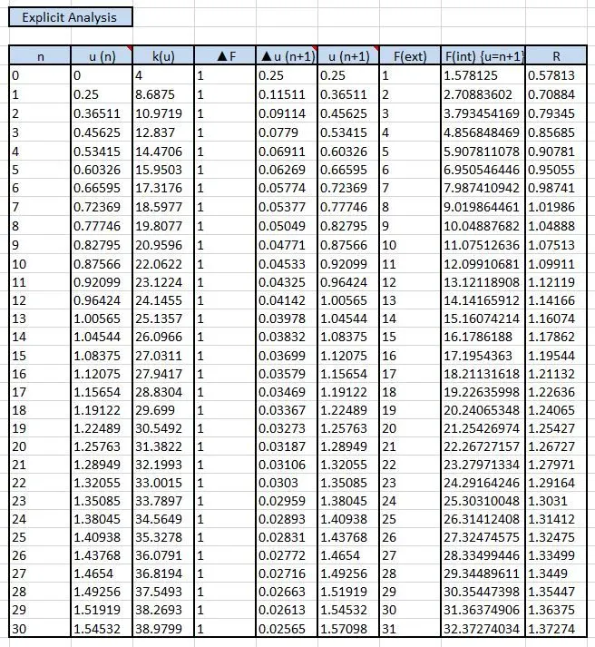
Explicit Analysis: Incremental displacements or incremental externally applied forces are represented as ∆u or ∆F. We will use an incremental load of ▲F at every step to calculate the variables displacement (u), Force (f), and residual (R).

Note: The solution below is just a manual calculation for describing the process. I have calculated this on the excel sheet so there the answers will vary due to approximations in manual calculations.

Using equation: ▲F=K▲u

Step-1: u0=0. Thus, k(u0)= 3*0*0+18*0+4=4

▲F=1. Thus, ▲u1=▲F/k(u0)=1/4=0.25

u1=u0+u1=0+0.25=0.25

Step-2: u1=0.25, k(u1)=3*0.25*0.25+18*0.25+4= 6.1875

▲F=1. ▲u2= ▲F/k(u1)=1/6.1875=0.162

u2=u1+▲u2=0.412

Similarly, by doing further iterations we can find out the displacement values.

Implicit Analysis: An implicit analysis is the same as the explicit analysis, except that at the end of each step Newton-Raphson iterations are used to enforce equilibrium before moving to the next step. Basically, an incremental force is applied to advance the solution forward at the beginning of a step. However, internal forces and external forces will not be in equilibrium unless the stiffness is linear for the given step. Hence, in order to achieve equilibrium, corrections must be made to the displacement. This is accomplished by using Newton-Raphson iterations to minimize the residual, R(u) = fint − Fext.

Note: The solution below is just a manual calculation for describing the process. I have calculated this on the excel sheet so there the answers will vary due to approximations in manual calculations.

Step-1: u0=0. Thus, k(u0)= 3*0*0+18*0+4=4

▲F=1. Thus, ▲u1=▲F/k(u0)=1/4=0.25

u1=u0+u1=0+0.25=0.25

Fext=▲F=1 and Fint=F(u at u=0.25)=1.578. R0=Fint-Fext=0.578 >0.01 (tolerance)

Thus, iteration is needed.

Iteration-1:

Δu1=-[k(0.25)]^-1*R0=-0.0665

u2= Δu1+u1=0.1835

Fext=▲F=1 and Fint=F(u at u=0.1835). R1=Fint-Fext=0.043 >0.01 (tolerance)

Thus, iteration is needed.

Iteration-2:

Δu2= Δu1-[k(0.25)]^-1*R1=-0.0072

u3= Δu2+u2 =0.178

Fext=▲F=1 and Fint=F(u at u=0.178). R1=Fint-Fext=0.0027 < 0.01 (tolerance)

Thus, no further iteration is needed.

Thus, the value is u1=0.178.

Similarly, we can do the further steps. And, as the implicit method has better convergence, we will get the same displacement values after a certain iteration.

In the above spreadsheet, I have put the K(u)2 value in the form of an if statement, i.e. if(R1<0.01,NA,3*u1^2+18u1+4) which means if R1 is less than 0.01 then say NA else calculate K(u)2 by the mentioned formula. Thus, the cells that show error is not actually a mistake but intentional to stop the calculation further as the residue is below tolerance.

Plotting Graphs:

First, calculate exact solutions by using the Goal seek method in excel.

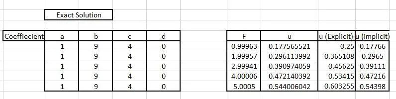
The displacement values in the column implicit and explicit are taken directly from the above spreadsheet for hassle-free plotting of the graphs.

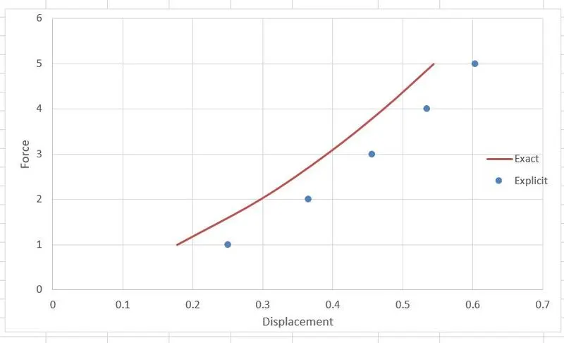
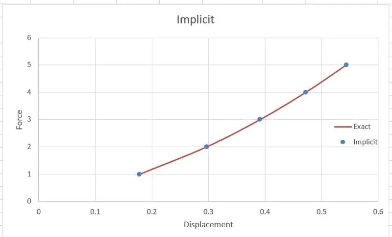
Remarks: This graph shows us clearly that the implicit method is much more precise than the explicit method thus taking more time for the solver to run the simulation. It also converges better with the exact solution than the explicit method.

CONCLUSION: Through this assignment, I have understood how a solver runs the simulations while employing implicit and explicit numerical methods. I have also understood the working and application of both methods.