Week - 2 - Explicit and Implicit Analysis

Part 1 – Implicit and explicit schemes.

Implicit and explicit schemes, as well as a combination of both, are numerical methods used to solve systems of differential equations for applications such as structural analysis. The origins of the words are important as they relate to how the numerical method is applied to solve the problem. Explicit refers to something that is clear and obvious, specific, and straight forward, while implicit refers to something that is inferred or assumed and not clear, specific, or obvious.

An explicit numerical equation is an equation where the unknown can be expressed solely on the left-hand side (LHS) and the right-hand side (RHS) contains items that are known. It can be viewed as a simple plug and chug equation.

An implicit numerical equation is an equation where the unknown in not expressed solely on the LHS. The unknown appears more than once in the equation and the equation cannot be algebraically rearranged so that the unknown can be expressed solely on the LHS with only known quantities on the RHS. In lieu of a plug and chug approach, it is typical to algebraically rearrange an implicit equation, so all terms are on the LHS and the RHS contains only the number zero. Then root finding techniques can be used to solve the equation.

The reasons that one scheme may be chosen over another for a particular problem include topics such as numerical stability, computational intensity and cost, the stiffness ratio of a differential equation, whether the equation is time-dependent or time-independent, whether a system of differential equations can be uncoupled, as well as others.

Part 2 – Aim of the challenge

The aim of this challenge is to demonstrate an understanding of the explicit and implicit numerical methods, both from a mathematical perspective and an application perspective where an intelligent decision can be made regarding which scheme to use to solve a particular structural analysis problem.

One method is not necessarily better than the other. One method may be more appropriate or better suited than the other depending on the particular problem that needs to be solved. In order to decide which method is more appropriate requires a thorough understanding of the problem.

If the problem is a dynamic impact, then acceleration is an important quantity. Typically, an explicit analysis is used for dynamic impacts. It is important to understand what the requirement is for the time step in an explicit analysis. If the time step becomes too small, the analysis becomes very computationally expensive. The time step in an explicit analysis has to be smaller than the time for a pressure wave to move through an element. So, the smallest element size in the mesh is very important. Creating a fine mesh can improve accuracy but also requires a smaller time step which is more computationally expensive. The time for a pressure wave to move through an element is based on the speed of sound through the material and the element size. When performing an explicit analysis, an engineer should always calculate the requirement on the time step prior to setting up and running the analysis. It is important to note that the explicit numerical method is not unconditionally stable. If the system of differential equations are stiff and/or the time step is too large, numerical instability can occur resulting in poor results. Below is the mathematical formulation for an explicit numerical method to solve a simple differential equation.

dy/dx = -y² – 2y

Let’s write this equation in discrete terms, where the dependent values on the RHS are considered at the current step k and the derivative on the LHS is in terms of step k and k+1.

(y_k+1 – y_k)/Dx = –y_k² – 2y_k

Now let’s algebraically rearrange the equation so the unknown at step k+1 is solely on the LHS and the RHS contains only known values at step k.

y_k+1 = y_k – Dx( y_k² + 2y_k)

This is an explicit numerical formulation for the differential equation.

If a problem is quasi-static or static, then acceleration is not considered. Typically, an implicit analysis is used for quasi-static or static events. The implicit numerical method is unconditionally stable. The time step requirements that are needed for an explicit analysis are not required for an implicit analysis. The down side of an implicit analysis is the solution technique requires additional process steps such as matrix inversion and root finding techniques which are computationally very expensive. The up side is that the time step can be increased resulting in fewer time steps to obtain a solution.

An example of an implicit technique would be to implement the trapezoidal rule, as shown below.

(y_k+1 – y_k)/Dx = 0.5*{(–y_k+1² – 2y_k+1) + (–y_k² – 2y_k)}

At the end of the day, the analysis engineer is interested in quality results at the lowest cost. The engineer must consider numerical stability, convergence to a quality solution, and the cost of computing by estimating the number of computing steps needed to obtain a solution. The number of computing steps is determined by not only the time step size but any intermediate computations required by an implicit technique. By making an engineering judgement to optimize all of the goals, the engineer can decide if an explicit or implicit analysis is more appropriate for the particular problem at hand.

Part 3. Given problem `f(u) = u^3 + 9u^2 = 4u`, `f(u=0)=0`

`f'(u) = 3u^2 + 18u + 4`

Explicit methodolgy: `frac{f_{i+1} - f_{i}}{u_{i+1} - u_{i}} = 3u_{i}^2+18u_{i}+4`

Explicit methodolgoy: `u_{i+1} = u_{i}+frac{f_{i+1}-f_{i}}{3u_{i}^2+18u_{i}+4}`

Implicit methodology: This is a multi-step method for each time step. First perform the explicit formula to obtain an estimate. Next, check the residual and iteratively calculate a correction until the magnitude of the residual is less than 0.001. I used a Force input in steps of unity with three time steps for a total input force of 3. I then calculated the displacement. Then check the residual and iteratively correct.

initial values for discrete analysis : `u_{i=1}=0 , k_{i=1}=4, F_{i=1}=0`

Now perform 3 time steps, increasing the force by 1 each step.

`F_{i+1}=F_{i}+1`

`u_{i+1}=u_{i}+frac{1}{k_{i}}*(F_{i+1}-F_{i})`

`f_{analytical}=u_{i+1}^3+9u_{i+1}^2+4u_{i+1}`

`R=f_{analytical}-F_{i+1}`

Do while abs(R)>0.001

`k=3*u_{i+1}^2+18u_{i+1}+4`

`u_{\text{correction}}=-1/k*R`

`u_{i+1}=u_{i+1}+u_{\text{correction}}`

Calculate new residual with corrected displacement

`f_{analytical}=u_{i+1}^3+9u_{i+1}^2+4u_{i+1}`

`R=f_{analytical}-F_{i+1}`

loop

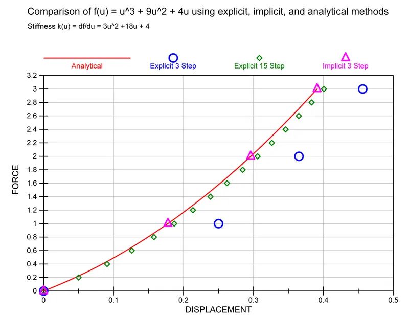
The results of peforming the 3 different analyses are shown on the plot below. I've also uploaded this plot as a PDF.

I performed the explicit analysis using 3 time steps (blue circles) and another explicit analysis using 15 time steps (green diamonds).

The explicit results are shown in purple triangles. The 3 time steps required 3, 3, and 2 iterations to obtain the required residual.

The analytical result is shown in red line.

The explicit method approaches the analytical results with smaller (more) time steps. It shows a converging solution but still has significant error.

The implicit method shows convergence with minimal error. I didn't calculate the number of floating point operations, but the implicit method required a total of 8 iterative steps plus 3 times steps for a total of 15 computation steps.