Challenge: WOT Condition

Aim:

1. Ratio of hill-climbing power required by fully loaded Tata ultra-truck to the half-loaded one.
2. Find the minimum length of the flyover, considering the minimum height at the summit should be 5.5 meters.
3. Prepare a new drive cycle excel file for the model and also include a hill-climbing angle to it.
4. Model the WOT (Wide Open Throttle) response of GM EV1 car. Prepare a table showing variation in acceleration time with a 5% change in vehicle parameters.

Study #1: -

Q1. Ratio of hill-climbing power required by fully loaded Tata ultra-truck to the half-loaded one.

Reference: https://light-trucks.tatamotors.com/light-trucks/tata-ultra/specifications/tata-ultra-t-12-light-trucks-specifications.aspx

Specifications of vehicle:

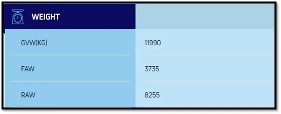
At full Load:-

Gross vehicle weight = kerb weight + payload weight = 3735 + 8255 = 11990 kg

Gradeability = 25.6% therefore, Angle = 15 degree

Hill climbing force = mass * gravity * sin (θ) = 11990 * 9.81 * sin(15) = 76448.1N

Consider velocity of the vehicle = 25kmph = 25*5/18 = 7 m/s

The hill climbing power can be calculated by the following formula:

Power = Hill Climbing Force * velocity of vehicle = 76448.1 * 7

Power at full load = 535136.7 W

At Half Load:-

Gross vehicle weight = kerb weight + payload weight/2 = 3735 + 8255/2 = 7862.5 kg

Hill climbing force = mass * gravity * sin (θ) = 7862.5 * 9.81 * sin(15) = 50157.45N

Consider velocity of the vehicle = 25kmph = 25*5/18 = 7 m/s

The hill climbing power can be calculated by the following formula:

Power = Hill Climbing Force * velocity of vehicle = 50157.45 * 7

Power at half load = 351102 W

Ratio of powers = (Power at full load) / (Power at half load) = `= (535136.7 )/351102 =`

1.524

Study #2: -

Q2. Find the minimum length of the flyover, considering the minimum height at the summit should be 5.5 meters.

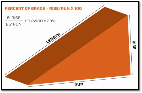
In this question, Rise = 5.5 meters

Angle (`θ`) = 15 degrees

Since it is a right angled triangle,

Sin (`θ`) = rise / length = sin (15) = 5.5 / length

Minimum Length of flyover = 21.25 meters

By Pythagoras Theorem;

Length² = Rise² + Run²

Minimum Run of the flyover = 20.5 meters

Study #3: -

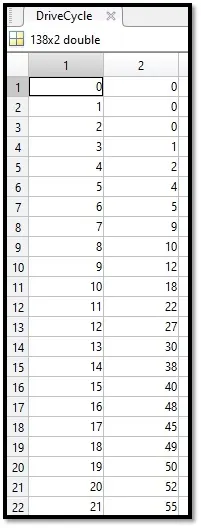
Q3. Prepare a new drive cycle excel file for the model and also include a hill-climbing angle to it.

New Drive Cycle Input:

Model: -

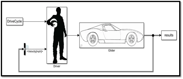
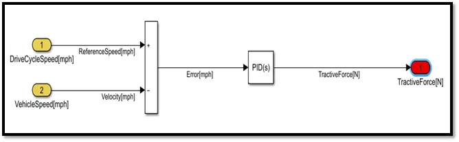
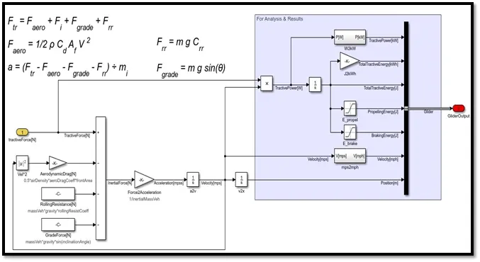
The instructions provided in the help section were followed and the Drive Cycle Excel sheet was imported into the Matlab workspace. Then in the Simulink model, the existing U.S drive cycle was replaced by the new one.

Driver Block: -

Glider Block: -

OUTPUT:

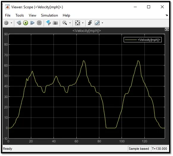
The Simulation was run for 138 seconds since there were 137 inputs in the drive cycle.

Study #4: -

Q4: Model the WOT (Wide Open Throttle) response of GM EV1 car. Compare it with the official figures of the performance of a real vehicle. Prepare a table showing variation in acceleration time with a 5% change in vehicle parameters.

Theory:

Wide open throttle (WOT) refers to an engine's maximum intake of air and fuel that occurs when the throttle plates inside the carburettor or throttle body are "wide open", providing the least resistance to the incoming air. In the case of an automobile, WOT is when the accelerator is depressed fully. In the case of a diesel engine, which does not have a throttle valve, WOT is the point at which the maximum amount of fuel is being injected relative to the amount of air pumped by the engine, generally in order to bring the fuel-air mixture up to the stoichiometric point.

Given GMEV data: -

Mass of vehicle = 1540kg

Drag Coefficient C_d = 0.19

Coefficient of rolling resistance µ_rr = 0.0048

Angular velocity = 733 rad/s

Gear ratio = 11

Efficiency of drive = 0.95

Tyre radius = 0.3m

Critical velocity = 19.8 m/s

Motor torque = 140 Nm

Motor Speed = 12000 rpm

Constant Power = 102kW

Maximum velocity = 35.8 m/s

Calculations:

`T= 102000/(37*v)= 2756/v`

Also,

F_te = F_rr + F_ad + F_la + F_wa

And `F= (T*G)/r`

Therefore,

`(T*G)/r= μ_rr*m*g+0.625AC_d v^2+(m+I G^2/(ƞ_g*r))* ((dv)/dt)`

Substituting and solving the given input values, we get:

`(dv)/dt=3.11-0.000137*v^2`

`(dv)/dt= 62.1/v-0.046-0.00317*v^2`

`v_(n+1)= v_n+ ∂t(3.11-0.000137v_n^2)`

`v_(n+1)= v_n+ ∂t(62.1/v_n -0.046-0.000137v_n^2)`

CODE:

clear all
close all
clc

t = linspace(0,20,201);
v = 0;
dt = 0.2;
for n = 1:200
    if v(n)<19.8
        v(n+1) = v(n)+ dt*(3.11-(0.000137*(v(n)^2)));
    elseif v(n)>=35.8
        v(n+1) = v(n);
    else
        v(n+1) = v(n)+ dt*((62.1/v(n))-0.046-(0.000137*(v(n)^2)));
    end
end

% Plotting
plot(t,v,'linewidth',3,'color','red');
xlabel("Time")
ylabel("Velocity")

Code Expaination:

The code contains a simple for loop in which there are three different conditions executed.

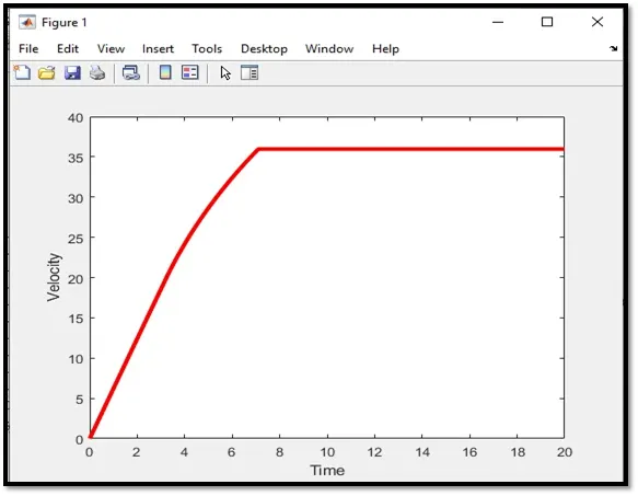
The two equations which were obtained by calculations are used for two conditions i.e, when velocity is less than the critical value (velocity < 19.8 m/s) and for velocity beyond the maximum value (velocity >= 35.8 m/s). The third condition is when the velocity of the vehicle lies between 19.8 & 35.8 m/s.

After executing it using "if-else" loop we finally plot the graph representing velocity vs time.

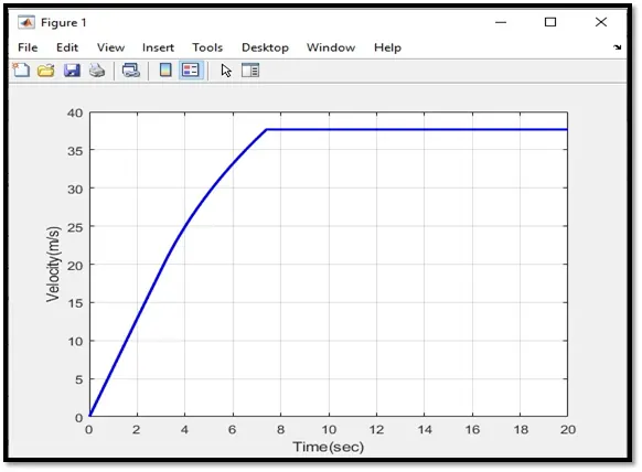
OUTPUT:

Changing the vehicle parameters by 5%: -

Mass of vehicle = 1617kg

Drag Coefficient C_d = 0.1995

Coefficient of rolling resistance µ_rr = 0.00504

Angular velocity = 769.65 rad/s

Gear ratio = 11

Efficiency of drive = 0.9975

Tyre radius = 0.315m

Critical velocity = 20.5 m/s

Motor torque = 147 Nm

Motor Speed = 12600 rpm

Constant Power = 107.1kW

Maximum velocity = 37.6 m/s

Solving for the above values, we get the following equations: -

`(dv)/dt=3.23-0.000152*v^2`

`(dv)/dt= 64.71/v-0.046-0.00152*v^2`

`v_(n+1)= v_n+ ∂t(3.23-0.000152v_n^2)`

`v_(n+1)= v_n+ ∂t(64.71/v_n -0.046-0.000152v_n^2)`

CODE:

clear all
close all
clc
t1 = linspace(0,20,201);
v1 = 0;
dt = 0.2;
for m = 1:200
    if v1(m)<20.5
        v1(m+1) = v1(m)+ dt*(3.23-(0.000152*(v1(m)^2)));
    elseif v1(m)>=37.6
        v1(m+1) = v1(m);
    else
        v1(m+1) = v1(m)+ dt*((64.71/v1(m))-0.046-(0.000152*(v1(m)^2)));
    end
end
% Plotting
plot(t1,v1,'linewidth',2,'color','blue');
xlabel("Time(sec)")
ylabel("Velocity(m/s)")
grid on

Code Explaination:

The same process was followed as the previous code. The equations and values of velocities were changed due to 5% increase in the input parameters.

OUTPUT:

Comparing the two outputs: -

CODE:

clear all
close all
clc

t = linspace(0,20,201);
v = 0;
dt = 0.2;
for n = 1:200
    if v(n)<19.8
        v(n+1) = v(n)+ dt*(3.11-(0.000137*(v(n)^2)));
    elseif v(n)>=35.8
        v(n+1) = v(n);
    else
        v(n+1) = v(n)+ dt*((62.1/v(n))-0.046-(0.000137*(v(n)^2)));
    end
end



t1 = linspace(0,20,201);
v1 = 0;
dt = 0.2;
for m = 1:200
    if v1(m)<20.5
        v1(m+1) = v1(m)+ dt*(3.23-(0.000152*(v1(m)^2)));
    elseif v1(m)>=37.6
        v1(m+1) = v1(m);
    else
        v1(m+1) = v1(m)+ dt*((64.71/v1(m))-0.046-(0.000152*(v1(m)^2)));
    end
end

% Plotting
plot(t,v,'linewidth',2,'color','red');
hold on
plot(t1,v1,'linewidth',2,'color','blue');
xlabel("Time(sec)")
ylabel("Velocity(m/s)")
grid on
legend('Original vehicle parameters','5% changed vehicle parameters')

OUTPUT:

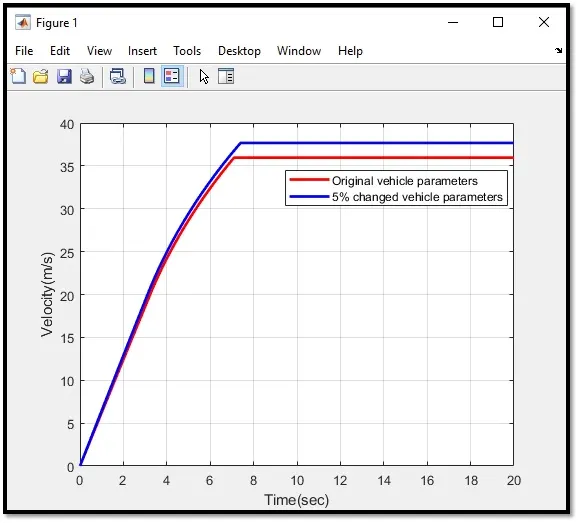
It is clearly evident from the plot that in both the cases, velocity of the vehicle remains constant after the maximum value.

In first case : velocity = 35.8 m/s

In second case : velocity = 37.6 m/s

CONCLUSIONS:

Thus we have sucessfully answered all the questions in this challenge with proper outputs and matlab code.

Study 1: - Ratio of powers = 1.524

Study 2: - Minimum Length of flyover = 21.25 meters

Study 3: - Graphical representation

Study 4: - Graphical representation