Week 2 Air standard Cycle

AIM: To write a program in python to solve an Otto cycle and plot its P-V diagram and output thermal efficiency.

Theory: The otto cycle is the ideal cycle for spark ignition reciprocating engines. In most spark-ignition engines, the piston executes four complete strokes(two mechanical cycles) within the cylinder, and the crankshaft completes two revolutions for each thermodynamic cycle.

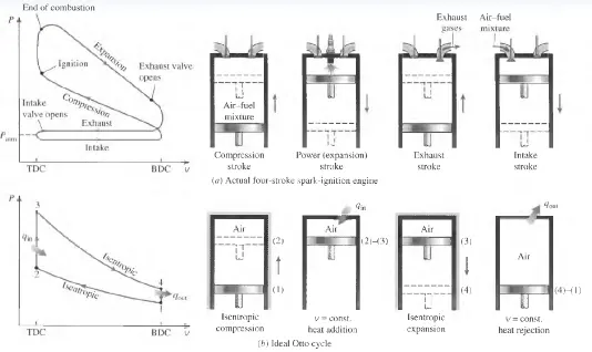
The four processes in an Otto cycle are:

1. isentropic compression process or reversible adiabatic compression of air (process 1-2),

2. Constant volume heat addition process (process 2-3),

3. Isentropic expansion process or reversible adiabatic expansion of air (process 3-4),

4. Constant volume heat rejection process (process 4-1).

GOVERNING EQUATION:

Various equations of the otto cycle are involved in this project are:

• Compression ratio (rc), rc= (V1V2) or 1+VsVc,
• Swept volume (Vs) = π4.d2.l, where d is bore diameter and I is stroke length,
• VVc = 1 + 12(rc-1)[R+1-cosθ-(R2-sin2θ)l2],

where R = length of connecting rod/crank radius,

• Adiabatic process equation = p.vγ = constant,
• Ideal gas equation = p.v = m.R.T,
• Thermal efficiency of the otto cycle(η) = 1-1rγ-1c,
• From the figure, v1 = vs + vc, c2=vc.

PYTHON CODE FOR SOLVING AND PLOTTING AIR STANDARD CYCLE:

#program by Srinithin
#Air standard cycle 
import numpy as np
import math
import matplotlib.pyplot as plt

def engine_kinematics(stroke, bore, con_rod, cr, start_crank, end_crank):

	#geometric para
	a = stroke/2
	R = con_rod/a

	#volume para
	v_s = math.pi*(1/4)*(bore**2)*stroke
	v_c = v_s / (cr-1)

	#Angles definition
	s_c = math.radians(start_crank)
	e_c = math.radians(end_crank)

	num_values = 50
	dtheta = (e_c-s_c)/(num_values)

	V=[]

	#for tracing the volume curve
	for i in range(0,num_values):
		theta = s_c + i*dtheta
		term1 = 0.5*(cr-1)
		term2 = R+1 - math.cos(theta)
		term3 = (pow(R,2)) - pow(math.sin(theta),2)
		term3 = pow(term3,0.5)
		V.append((1+term1*(term2-term3))*v_c)
	return V


#inputs
p1 = 101325
t1 = 500
gamma = 1.4
t3 = 2300

#geometric para
bore = 0.1
stroke = 0.1

#connecting rod length
con_rod = 0.15

#compression ratio
cr = 12

#volume computation
#v_c = clearance volume, v_s = swept volume
#state point 1(isentropic compression process)

v_s = (math.pi/4)*(bore**2)*stroke
v_c = v_s/(cr-1)
v1 = v_c + v_s

"""
state point2 (constant volume heat addition process)
"""
v2 = v_c

# p2v2^gamma = p1v1^gamma
p2 = p1*(v1**gamma)/(v2**gamma)

#ideal gas law
#p1v1/t1 = p2v2/t2 | rhs=p1v1/t1 |rhs = p2v2/t2 | t2=p2v2/rhs
rhs = (p1*v1)/t1
t2 = (p2*v2)/rhs
V_comp = engine_kinematics(bore, stroke, con_rod, cr, 180, 0)

constant = p1*(v1**gamma)

p_comp = []
for V in V_comp:
	p_comp.append(constant/(V**gamma))

#state point 3 (isentropic expansion process)
v3 = v2

#p2v2/t2 = p3v3/t3 | rhs=p2v2/t2 | p3=rhs*t3/v3

rhs = p2*v2/t2

p3 = (rhs*t3)/v3

v_expansion = engine_kinematics(bore, stroke, con_rod, cr,0,180)
constant = p3*(v3**gamma)

p_expansion = []
for V in v_expansion:
	p_expansion.append(constant/(V**gamma))

#state point 4 (const vol heat rejection process)
v4=v1
#p4v4^gamma = p3v3^gamma
p4 = p3*(v3**gamma)/(v4**gamma)

#p4v4/t4=rhs
t4=p4*v4/rhs

#plotting PV diagram
plt.plot([v2,v3],[p2,p3])
plt.plot(V_comp,p_comp)
plt.plot(v_expansion,p_expansion)
plt.plot([v4,v1],[p4,p1])
plt.xlabel('Volume [m^3]')
plt.ylabel('Pressure [Pa]')
plt.title('P-V diagram of an otto cycle')
plt.grid()
plt.show()

#thermal efficiency of Engine
n = 1-(cr**(1-gamma))
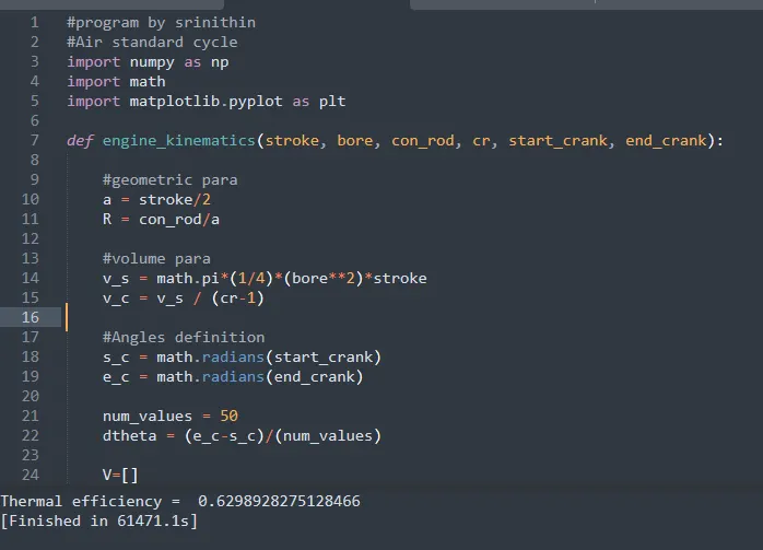
print("Thermal efficiency = ", n)

RESULT:

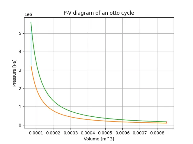
• Upon executing the above program, the following plot for the P-V curve was observed.

THERMAL EFFICIENCY OUTPUT:

CONCLUSION:

• Plotted the PV diagram for the respective input using an array of volumes inside the engine cylinder at different crank angles.
• Thermal efficiency calculation is output.