Week 2 Air standard Cycle

"""

Otto cycle simulator

"""

import math
import matplotlib.pyplot as plt

# Inputs
p1 = 101325
t1 = 500
t3 = 2300
gamma = 1.4

# Geometric parameters
bore = 0.1
stroke = 0.1
con_rod = 0.15
cr = 4

# Volume computation
v_s = (math.pi/4)*pow(bore,2)*stroke
v_c = v_s/(cr-1)
v1 = v_s + v_c

# State point 2
v2 = v_c

# p2v2^gamma = p1v1^gamma
p2 = p1*pow(v1,gamma)/pow(v2,gamma)

#p2v2/t2 = p1v1/t1 | rhs = p1v1/t1 | p2v2/t2 = rhs | t2 = p2v2/rhs
rhs = p1*v1/t1
t2 = p2*v2/rhs


# state point 3
v3 = v2

#p3v3/t3 = p2v2/t2 | rhs = p2v2/t2 | p3 = rhs*t3/v3
rhs = p2*v2/t2
p3 = rhs*t3/v3

# State point 4
v4 = v1

#p4v4^gamma = p3v3^gamma

p4 = p3*pow(v3,gamma)/pow(v4,gamma)

#p4v4/t4 = p3v3/t3 | p4v4/t4 = rhs
 
t4 = p4*v4/rhs

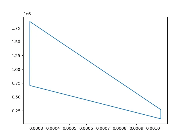
plt.plot([v1,v2,v3,v4,v1],[p1,p2,p3,p4,p1])
plt.show()

# Thermal efficiency
Eta_thermal = [1-((t4-t3)/(t2-t1))]

print(t1,t2,t3,t4)
print(Eta_thermal)