Week 2 Air standard Cycle

Aim:-

Write a program in python that can solve an otto cycle and make plots for it.

Objective:-

Create a PV diagram.

The code should be able to output the thermal efficiency of the engine.

Softwares Used:-

Python 3.8

Sublime Text 4

Google Docs

Governing Equations:-

Otto cycle:-

Assuming ideal gas

1-2: Air-fuel mixture is compressed isentropically.

2-3: Heat is added in an instantaneous constant volume process.

3-4: High Temperature and high-pressure gas are allowed to expand isentropically to produce work.

4-1: Heat is rejected in a constant volume process.

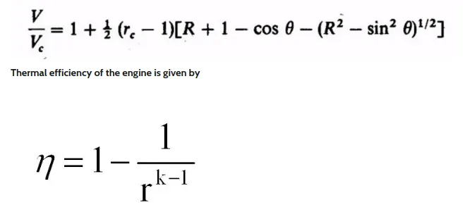
where ,

= Thermal Efficiency

r = (compression ratio)

k = gamma = 1.4

Body of the content:-

import math
import matplotlib.pyplot as plt

def engine_kinematics(bore,stroke,con_rod,cr,start_crank,end_crank):
	"""
	Engine Kinematics
	"""

	#Geometric parameters
	a = stroke/2
	R = con_rod/a

	# Volume parameters
	# V_s & V_c are swept volume and clearance volume respectively
	v_s = (math.pi/4)*pow(bore,2)*stroke
	v_c = v_s/(cr-1)

	sc = math.radians(start_crank)
	ec = math.radians(end_crank)

	num_value = 100

	dtheta = (sc-ec)/(num_value - 1)
	#print(dtheta)

	v = []

	for i in range(0,num_value):

		#print(i)
		
		theta = sc + i*dtheta
		#print(theta)
		term1 = 0.5*(cr - 1)
		term2 = R + 1-math.cos(theta)
		term3 = (pow(R,2) - pow(math.sin(theta),2))
		term4 = pow(term3,0.5)

		v.append((1 + term1*(term2 - term4))*v_c)

	return v
		
#inputs 
#Pressure(Pa)
p1 = 101325

#Temperature (K)
t1 = 500
t3 = 2300

#specific heat ratio
gamma = 1.4

#geometric parameters (m)
#Square engine
bore = 0.1
stroke = 0.1

#connecting Rod(m)
con_rod = 0.15

#compression ratio
cr = 8

# Volume compensation
v_s = (math.pi/4)*pow(bore,2)*stroke
v_c = v_s/(cr-1)

v1 = v_c + v_s

# State point 2

v2 = v_c

# p2v2^gamma = p1v1^gamma

p2 = p1*pow(v1,gamma)/pow(v2,gamma)


#p2v2/t2 = p1v1/t1
#const = p1v1/t1 = p2v2/t2
#t2 = p2v2/const

const = p1*v1/t1	
t2 = p2*v2/const

v_compression = engine_kinematics(bore,stroke,con_rod,cr,180,0)
constant = p1*pow(v1,gamma)

p_compression = []

for v in v_compression:
	p_compression.append(constant/pow(v,gamma))


#state 3 

v3 = v2

#p3v3/t3 = p2v2/t2
#const= p2v2/t2, p3 = const*t3/v3

const = p2*v2/t2
p3 = const*t3/v3

v_expansion = engine_kinematics(bore,stroke,con_rod,cr,0,180)

constant = p3*pow(v3,gamma)

p_expansion = []

for v in v_expansion:
	p_expansion.append(constant/pow(v,gamma))

# state point 4

v4 = v1

# p4v4^gamma = p3v3^gamma
p4 = p3*pow(v3,gamma)/pow(v4,gamma)

# p4v4/t4 = const

t4 = (p4*v4)/const

#Thermal efficiency

n = 1 - (pow(cr,(1-gamma)))
print(n)

plt.figure(1)
plt.plot([v2,v3],[p2,p3])
plt.plot(v_compression,p_compression)
plt.plot(v_expansion,p_expansion)
plt.plot([v4,v1],[p4,p1])
plt.title('P-V Diagram for otto cycle')
plt.xlabel('Volume(m^3/s)')
plt.ylabel('Pressure(Pa)')
plt.show()

Results and Discussions:-

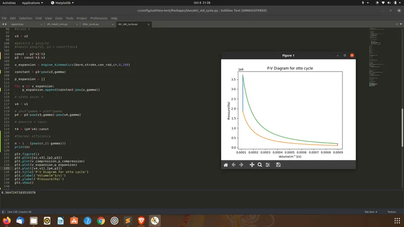
#Output for Program

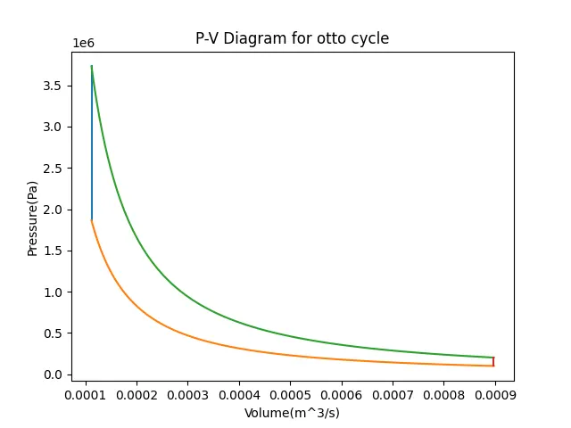
(Thermal Efficiency) = 56.47%

Conclusions:-

P-V diagram is plotted for the ideal otto cycle.