Week 2 Air standard Cycle

OBJECTIVE : In this report i have to write the python code for otto cycle , the code should plot the pv diagram based on otto cycle and also we will get the efficiency of the engine as result of the program.

PROBLEM STATEMENT : All the engines runs on petrol are based on the otto cycle. Mainly the otto cycle has processes defined below:

PROCESS 1. A mass of air is drawn in to piston/cylinder arrangement at constant pressure (SUCTION STROKE)

PROCESS 2. It is an reversible adiavatic (isentropic) compression of the charge as the piston moves from bottom dead center (BDC) to the top dead center (TDC). (COMPRESSION STROKE)

PROCESS 3. It is an constant volume heat transfer to the working gas from an external source while the piston is at the top dead center (TDC). This process is intended to represent the ignition of the fuel-air mixture and the subsequent burning.(CONSTANT VOLUME HEAT ADDITION)

PROCESS 4. It is an reversible adiavatic (isentropic) expansion process , in which piston moves back from top dead center to bottom dead center. (POWER STROKE)

PROCESS 5. It is an constant volume heat rejection in which heat is rejected though the system by an external source (such as coolant )

PROCESS 6. It is a process in which burnt gases are through out from the system through the valves open. (EXHAUST STROKE)

This is the basic explanation of the otto cycle and four stroke engines (petrol engines). We will use relations based on these processes to find a logic of our program.

SOLUTION PROCEDURE:

python program for otto cycle:

import math
import matplotlib.pyplot as plt


def engine_kinematics(bore,stroke,con_rod,cr,start_crank,end_crank):

	a = stroke/2
	R = con_rod/a
	V = []
	# volume parameters
	v_s = (math.pi/4)*pow(bore,2)*stroke
	v_c = v_s/(cr-1)

	sc = math.radians(start_crank)
	ec = math.radians(end_crank)


	num_values = 50

	dtheta = (ec-sc)/(num_values-1)
	 

	for i in range(0,num_values):
		theta = sc + i*dtheta
		


		term1 = 0.5*(cr-1)
		term2 = R+1-math.cos(theta)
		term3 = pow(R,2) - pow(math.sin(theta),2)
		term3 = pow(term3,0.5)

		V.append((1+term1*(term2-term3))*v_c)
	return V

# inputs
p1 = 101325
t1 = 500
gamma = 1.4
t3 = 2300

# geometric parameters
bore = 0.1
stroke = 0.1
con_rod = 0.15
cr = 12

# volume computations
v_s = (math.pi/4)*(pow(bore,2))*stroke
v_c = v_s/(cr-1)
v1 = v_c + v_s

# state point 2

v2 = v_c

# p1v1^gamma = p2v2^gamma
p2 = p1*pow(v1,gamma)/pow(v2,gamma)

# p2v2/t2 = p1v1/t1 | rhs = p1v1/t1 | p2v2/t2 = rhs | t2 = p2v2/rhs
rhs = p1*v1/t1
t2 = p2*v2/rhs

V_compression = engine_kinematics(bore,stroke,con_rod,cr,0,180)

constant = p1*pow(v1,gamma)

P_compression = []
for v in V_compression:
	P_compression.append(constant/pow(v,gamma))


# state point 3

v3 = v2

# p3v3/t3 = p2v2/t2 | rhs = p2v2/t2 | p3v3/t3 = rhs | p3 = rhs*t3/v3
rhs = p2*v2/t2
p3 = rhs*t3/v3

V_expansion = engine_kinematics(bore,stroke,con_rod,cr,180,0)

constant = p3*pow(v3,gamma)

P_expansion = []
for v in V_expansion:
	P_expansion.append(constant/pow(v,gamma))

# state point 4

v4 = v1

# p4v4^gamma = p3v3^gamma

p4 = p3*(pow(v3,gamma))/pow(v4,gamma)

# p4v4/t4 = p3v3/t3

t4 = p4*v4/rhs
# thermal efficiency of the engine (based on otto cycle)

# relation for the efficiency (eeta) = 1-1/cr^(gamma-1)

eeta = 1 - 1/pow(cr,(gamma-1))

print (eeta)
plt.plot([v2,v3],[p2,p3])
plt.plot(V_compression,P_compression)
plt.plot(V_expansion,P_expansion)
plt.plot([v4,v1],[p4,p1])
plt.show()

EXPLANATION:

1. Starting from importing the math and matplotlib library because we are using math function and plotting of graphs.
2. After that defining a function engine_kinematics has a set (bore,stroke,con_rod,cr,start_crank,end_crank)
3. Introducing the variables a = crank pin radius, R = constant V is introduced as an empty array.
4. Having the swept volume and clearance volume by the relation v_s = (math.pi/4)*pow(bore,2)*stroke , v_c = v_s/(cr-1)
5. Having starting and end crank angle sc = math.radians(start_crank) , ec = math.radians(end_crank)
6. Having no. of values 50 for isentropic compression and expansion.
7. dtheta is known as the intervals between the theta value
8. Introducing for loop for i in range(0,num_values):
9. For crank angle theta = sc + i*dtheta
10. For getting the volume trace we use the farmula which we devided in to terms as term1 = 0.5*(cr-1)
    term2 = R+1-math.cos(theta)
    term3 = pow(R,2) - pow(math.sin(theta),2)
    term3 = pow(term3,0.5)
11. now appending the empty array V to the relation we have, V.append((1+term1*(term2-term3))*v_c)
12. After calculating command the function that return the value of V return V
13. Introducing the state variables for point 1 using the basic process relation we have

    # inputs
    p1 = 101325
    t1 = 500
    gamma = 1.4
    t3 = 2300

    # geometric parameters
    bore = 0.1
    stroke = 0.1
    con_rod = 0.15
    cr = 12

    # volume computations
    v_s = (math.pi/4)*(pow(bore,2))*stroke
    v_c = v_s/(cr-1)
    v1 = v_c + v_s

14. for compression process we have to calculate the pressure and volume trace for compression process as how it changes for crank different crank angle is defined by the v_compression and p_compression

    # state point 2

    v2 = v_c

    # p1v1^gamma = p2v2^gamma
    p2 = p1*pow(v1,gamma)/pow(v2,gamma)

    # p2v2/t2 = p1v1/t1 | rhs = p1v1/t1 | p2v2/t2 = rhs | t2 = p2v2/rhs
    rhs = p1*v1/t1
    t2 = p2*v2/rhs

    V_compression = engine_kinematics(bore,stroke,con_rod,cr,0,180)

    constant = p1*pow(v1,gamma)

    P_compression = []
    for v in V_compression:
    P_compression.append(constant/pow(v,gamma))

15. Same as above we calculate for the state variables for point 3, also have to calculate the v_expansion and p_expansion

    # state point 3

    v3 = v2

    # p3v3/t3 = p2v2/t2 | rhs = p2v2/t2 | p3v3/t3 = rhs | p3 = rhs*t3/v3
    rhs = p2*v2/t2
    p3 = rhs*t3/v3

    V_expansion = engine_kinematics(bore,stroke,con_rod,cr,180,0)

    constant = p3*pow(v3,gamma)

    P_expansion = []
    for v in V_expansion:
    P_expansion.append(constant/pow(v,gamma))

16. same as for state point 4 ,

    # state point 4

    v4 = v1

    # p4v4^gamma = p3v3^gamma

    p4 = p3*(pow(v3,gamma))/pow(v4,gamma)

    # p4v4/t4 = p3v3/t3

    t4 = p4*v4/rhs

17. for efficiency of the otto cycle we use the coding as

    # thermal efficiency of the engine (based on otto cycle)

    # relation for the efficiency (eeta) = 1-1/cr^(gamma-1)

    eeta = 1 - 1/pow(cr,(gamma-1))

RESULTS AND DISCUSSION :

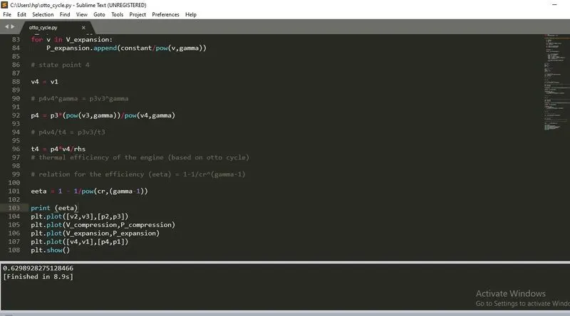
Here is the result of the program i.e efficiency of the otto cycle is 62.98%

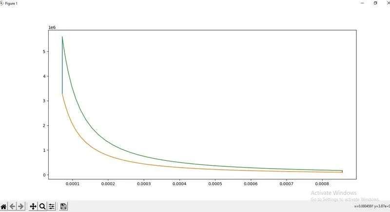
Here it is shown the PV Diagram of otto cycle and based on our program result