Week 2 Air standard Cycle

Objective:

Write a code that can solve an otto cycle and make plots for it.

Otto Cycle :

• Process 0–1 a mass of air is drawn into piston/cylinder arrangement at constant pressure.
• Process 1–2 is an adiabatic (isentropic) compression of the charge as the piston moves from bottom dead center (BDC) to top dead center (TDC).
• Process 2–3 is a constant-volume heat transfer to the working gas from an external source while the piston is at top dead center. This process is intended to represent the ignition of the fuel-air mixture and the subsequent rapid burning.
• Process 3–4 is an isentropic expansion (power stroke).
• Process 4–1 completes the cycle by a constant-volume process in which heat is rejected from the air while the piston is at bottom dead center.
• Process 1–0 the mass of air is released to the atmosphere in a constant pressure process.

Steps followed to write a code:

1. Import math and matplotlib.pyplot as plt

2. Define a function with function name and pass the arguments through it.

3. Calculate for Volume at different crank angles and store the values of volume in an array.

4. Define the thermodynamic properties at four different points using the relation:

pvt=constant

5. Plot the thermodynamic processes using the command plot.plt('variable names ')

6. Define the thermal efficiency of the engine.

Code:

# Program to write otto cycle simulator 
import math 
import matplotlib.pyplot as plt 
# inputs  


def engine_kinematics(bore,con_rod,stroke,cr,start_crank,end_crank):
	
	"""

	Engine Kinematics

	"""
	# Defining the  Geometric Parameters 
	a=stroke/2
	R=con_rod/a

	# Volume Parameters
	V_s= math.pi*(1/4)*pow(bore,2)*stroke    
	V_c=V_s/(cr-1)
    # Starting and ending crank angle 
	sc=math.radians(start_crank) # Denotes starting crank and ending crank 
	ec=math.radians(end_crank)
     
	num_values=100 
	dtheta=(ec-sc)/(num_values-1)
	V=[] # Storing the values of volume at different crank angles 
	for i in range(0,num_values ):
		theta=sc+i*dtheta
		term1=0.5*(cr-1)
		term2=R+1-math.cos(theta)
		term3=pow(R,2)-pow(math.sin(theta),2)
		term3=pow(term3,0.5)	
		V.append((1+term1*(term2-term3))*V_c)

	return V
	
# state point 1 
p1=101325
t1=500
gamma=1.4
t3=2300

# geometric parameters 
bore=0.1
stroke=0.1
con_rod=0.15	
cr=12

# Volume Computation 
v_s=(math.pi/4)*pow(bore,2)*stroke
v_c=v_s/(cr-1)
v1=v_c+v_s

# state point 2 
v2=v_c
# p2v2^gamma=p1v1^gamma
p2=p1*pow(v1,gamma)/pow(v2,gamma)

# p2v2/t2=p1v1/t1 | rhs=p1v1/t1 | p2v2/t2 =rhs | t2=p2v2/rhs
rhs=p1*v1/t1
t2=p2*v2/rhs
V_compression=engine_kinematics(bore,con_rod,stroke,cr,180,0)

constant=p1*pow(v1,gamma)                                                                                                                                      
P_compression=[]
for v in V_compression:
	P_compression.append(constant/pow(v,gamma)) 

# state point 3 
v3=v2 
# p3v3/t3=p2v2/t2  |  rhs=p2v2/t2 | p3=rhs*t3/v3
rhs=p2*v2/t2
p3=rhs*t3/v3
V_expansion=engine_kinematics(bore,con_rod,stroke,cr,0,180)

constant=p3*pow(v3,gamma)                                                                                                                                      
P_expansion=[]
for v in V_expansion:
	P_expansion.append(constant/pow(v,gamma)) 


# state point 4 
v4=v1
#p4*v4^gamma= p3*v3^gamma
p4=p3*pow(v3,gamma)/pow(v4,gamma)
# p4v4/t4=rhs
t4=p4*v4/rhs 

plt.plot([v2,v3],[p2,p3])
plt.plot(V_compression, P_compression)
plt.plot(V_expansion, P_expansion)
plt.plot([v4,v1],[p4,p1])
plt.xlabel('volume') # label for X-axis
plt.ylabel('pressure') # label for Y-axis 

plt.show() # To show a plot

thermalefficiency = (1-(1/pow(cr,(gamma-1))))*100
print(thermalefficiency)

Output:

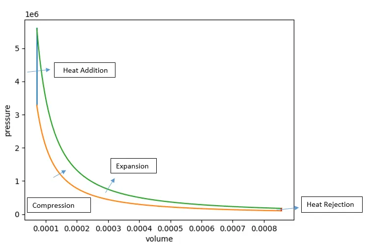
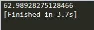
Thermal Efficiency of the Engine

Conclusion:

As it could be seen from above results that plot for the PV Diagram has been generated using the above code and the thermodynamic processes has been displayed in the graph as shown .Thermal Energy of the engine has been calculated as displayed above.