Week 2 Air standard Cycle

A Python program to plot a PV diagram for an otto cycle.

Aim -

• To plot the PV diagram of an otto cycle by finding the State variables
• Given inputs are variables of the cylinder which include bore, stroke

Briefing

• Otto cycle helps to understand the functioning, process, and different states during the thermodynamic events in an Internal Combustion engine.

• Understand the working of an IC engine can help better understand the PV plot of an Engine.
• During process 0–1, a mass of air is drawn into the piston/cylinder arrangement at constant pressure.
• Process 1–2 is an adiabatic (isentropic) compression of the charge as the piston moves from the bottom dead center (BDC) to top dead center (TDC).
• Process 2–3 is a constant-volume heat transfer to the working gas from an external source while the piston is at the top dead center. This process is intended to represent the ignition of the fuel-air mixture and the subsequent rapid burning.
• Process 3–4 is an adiabatic (isentropic) expansion (power stroke).
• Process 4–1 completes the cycle by a constant-volume process in which heat is rejected from the air while the piston is at the bottom dead center.
• Process 1–0 the mass of air is released to the atmosphere in a constant pressure process.

Procedure to generate a code the PV plot of the typical otto cycle

Challenges :

• Since the compression and expansion processes are not linear the pressure and volume values need to find out changing crank angle

Steps :

• Initially, we inputting the values which are given
  
  • bore
  • stroke
  • connecting rod length
  • compression ratio
  • gamma
• Based on this we find out the swept and clearance volume of the cylinder.
• Then we input state 1 variables which are pressure, temperature, and volume.
• Using ideal gas law we find the unknown variables.
• During the compression process. volume decreases, and pressure increases, by inputting the crank angle for compression, a volume function is called where 50 points for degrees between the crank angles are used to calculate the volume changes for each point.
• This volume compression array is then used to calculate compression process pressure.
• Similarly, for the expansion process, the volume and pressure values are found out.
• Thermal effiecny is then calculated using this formulae : 1-((t_4-t_1)/(t_3-t_2))
• Plotting: first the heat addition process is plotted and then the compression and expansion values are plotted.
• In the end, the heat rejection process is plotted using the state 4 values.

#program to simulate air std cycle. 

import math
import matplotlib.pyplot as plt

def engine_volume(b,stroke,con_rod,cr,start_angle,end_angle):

	a = stroke/2 # crank pin radius
	R = con_rod/a # Constant

	v_s = math.pi*(1/4)*pow(bore,2)*stroke # swept volume
	v_c = v_s/ (cr-1) # 

	sc = math.radians(start_angle)
	ec = math.radians(end_angle)

	num_values =  50
	dtheta = abs( (ec-sc)/(num_values-1)) # dividing the angles into smallest equal parts

	V = []
	for i in range(0,num_values):

		theta = sc*i*dtheta

		term_1 = 0.5*(cr-1)
		term_2 = R + 1 - math.cos(theta)
		term_3 = pow( pow(R,2) - pow(math.sin(theta),2) , 0.5 )
		volume = (1 + term_1*(term_2-term_3))*v_c
		
		V.append(volume)
	return V

#geometric parameters
bore = 0.1
stroke  = 0.1
con_rod = 0.15
cr = 12 # compression ratio

#volume paramters
v_s = math.pi*(1/4)*pow(bore,2)*stroke # swept volume
v_c = v_s/ (cr-1) # clearance volume

#intial state 1 values >> assumption 
p_1 = 10000
t_1 = 500 
v_1 = v_s + v_c
gamma = 1.4
t_3 = 2300 # constant volume heat addtion assumtion > combustion happens

# State 2 compression
v_2 = v_c
constant_1 = p_1*pow(v_1,gamma)
p_2 = constant_1/pow(v_2,gamma)
print(p_2)
# gas law p1*v1/t1 = p2*v2/t2
rhs = p_1*v_1/t_1
t_2 = p_2*v_2/rhs

#finding the values of volume for 180 to 0 >> connecting
V_compression = engine_volume(bore,stroke,con_rod,cr,180,0)
#def engine_volume(b,stroke,con_rod,cr,start_angle,end_angle):

#finding the values of pressure compression
P_compression = []
for v in V_compression:
	P_compression.append(constant_1/pow(v,gamma))

# State 3 contant volume
v_3 = v_2
rhs = p_2*v_2/t_2
p_3 = rhs*t_3/v_3

print(p_3)

V_expansion = engine_volume(bore,stroke,con_rod,cr,270,360)
constant = p_3*pow(v_3,gamma)

print(V_expansion)

P_expansion = []

for x in V_expansion:
	P_expansion.append(constant/pow(x,gamma))

# State 4 
v_4 = v_1
p_4 = p_3*pow(v_3,gamma)/pow(v_4,gamma)
t_4 = p_4*v_4/rhs

#thermal efficiency

n = 1-((t_4-t_1)/(t_3-t_2))

print('thermal efficiency % = ',n*100)

plt.grid()

plt.plot([v_2,v_3],[p_2,p_3])
plt.plot(V_compression,P_compression)
plt.plot(V_expansion,P_expansion)
plt.plot([v_4,v_1],[p_4,p_1])
plt.title("Pressure vs Volume Plot for Otto cycle")
plt.xlabel("Volume")
plt.ylabel("Pressure")
plt.show()

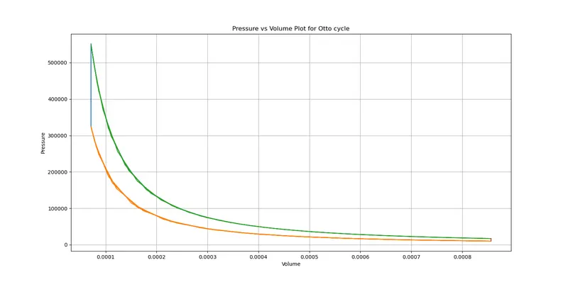
Results:

• The PV plot of an Otto cycle helps in determining the peak pressure in an IC engine.
• Just by inputting various values of engine parameters the efficiency of an engine can be found out, in this case, the thermal efficiency is 62.98%.