Week 2 Air standard Cycle

AIM: generate the otto cycle and find efficiency in python.

• we can divide the methodology into given parts

Methodology

• Otto cycle
• Otto cycle stages
• Python code & results
• Explanation
• Learning outcome

Otto cycle

There are two main parts to engine operation: the mechanical operation of the engine parts, and the thermodynamics through which the engine produces work and power.

In an internal combustion engine, fuel and air are ignited inside a cylinder. The hot exhaust pushes a piston which is connected to a crankshaft to produce power. The burning of fuel is not a continuous process but occurs very quickly at regular time intervals. Between ignitions, the engine parts move in a repeated sequence called a cycle. the engine is called four-stroke engine. otto cycle contains same characteristics.

Otto cycle stages

there are four-cycle contains in otto cycle.

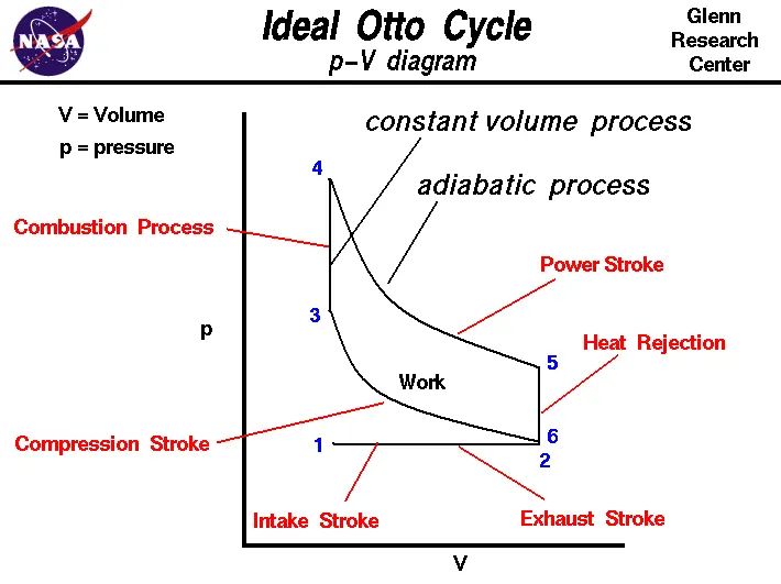
1)compression stroke(adiabatic process)

2)combustion process

3) expansion stroke(adiabatic process)

4)heat rejection

for adiabatic process

`pv^gamma=constant`

Ideal gas law

`pv=nrt`

we will solve the combustion chamber volume related to the adiabatic process.

Python code

"""otto cycle simulator
	by  dhanik
	"""
import math
import matplotlib.pyplot as plt


def engine_kinematics(bore,stroke,con_rod, cr, start_theta, end_theta):
	

	#parameters

	v_s=(math.pi/4)*(pow(bore,2))*stroke #swept volume
	v_c=v_s/(cr-1)

	crank_pin_radius=stroke/2
	R=con_rod/crank_pin_radius
	n=10
	et=90
	st=0
	theta=[]
	V=[]
	st=math.radians(start_theta)
	et=math.radians(end_theta)
	dtheta=(et-st)/(n-1)
	for i in range(0,n):
		theta=st+i*dtheta
	
		#print(theta)

		term1=0.5*(cr-1)
		term2=R+1-math.cos(theta)
		term3=pow(R,2)-pow(math.sin(theta),2)
		term3=pow(term3,0.5)
		V.append((1+term1*(term2-term3))*v_c)
	return V

#inputs
p1=101325 #in pascal
t1=500 #in kelvin
gamma=1.4
t3=2300

	
#geomatric parameters
bore=0.1 #in meter
stroke=0.1
con_rod=0.15
cr=12

#volume for 1 st state point
v_s=(math.pi/4)*(pow(bore,2))*stroke #swept volume
v_c=v_s/(cr-1)
v1=v_c+v_s

#print(v_c)

#volume for state point 2
v2=v_c
#p1v1^gamma=p2v2^gamma
p2=p1*pow(v1,gamma)/pow(v2,gamma)
#print(p2)
#defining new varibale for easiness
a=p1*v1/t1
#p2v2/t2=p1v1/t1
t2=p2*v2/a
print(t2)
V_compression=engine_kinematics(bore,stroke,con_rod, cr, 180,0)
constant=p1*pow(v1,gamma)
#print(constant)
P_compression=[]
print(V_compression)

for v in V_compression:
	P_compression.append(constant/pow(v,gamma))
print(P_compression)

#print(t2)

#state point 3
v3=v2
a=p2*v2/t2
#p3v3/t3=p2v2/t2
p3=a*t3/v3
#print(p3)
constant=p3*pow(v3,gamma)

V_expansion=engine_kinematics(bore,stroke,con_rod, cr, 0,180)

P_expansion=[]
print(V_expansion)

for v in V_expansion:
	P_expansion.append(constant/pow(v,gamma))
print(P_expansion)

#state point 4
v4=v1
p4=p3*pow(v3,gamma)/pow(v4,gamma)
a=p3*v3/t3
t4=p4*v4/a
print(t4)
#print(p3)

#finding efficiency
efficiency=(1-((t4-t1)/(t3-t2)))*100
print(efficiency)

plt.plot((v2,v3,),(p2,p3),label='heat additon process')
plt.plot(V_compression,P_compression,label='compression process',marker='o')
plt.plot(V_expansion,P_expansion,label="expansion process",marker='*')
plt.plot((v4,v1,),(p4,p1),label="heat rejection process")
plt.xlabel('volume')
plt.ylabel('pressure')
plt.legend()
plt.show()

code and result explanation

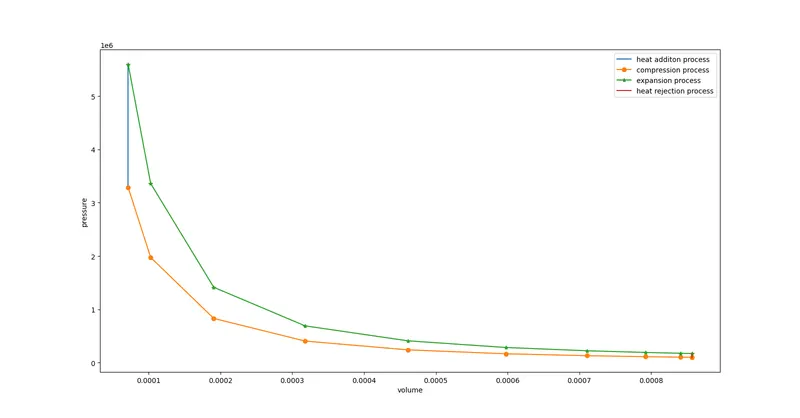
• Created a function in code for easiness, where variables, inputs, and geometric parameters are defined. after that, variables for different states such as pressure-volume and temperature are defined by using standard formulas.
• the adiabatic process is a nonlinear process where pressure and volume both are changing. for compression when air is entering in the engine chamber volume is shrinking and volume is decreasing, however, for the expansion, it is completely opposite. whereas the other two processes are utterly constant volume processes, but the temperature is changing. here this diagram of the ideal Otto cycle.
• volume and pressure are calculated for 10 values, by changing slightly in code individual can get a smooth curve.
• Here, t1 and t3 are assumed to find efficiency.
• Efficiency formula

• thermal efficiency =62%

learning outcome

• Making a function and calling function
• for loop use
• otto cycle basis and generating a graph with detail.