CREATE A AIR STANDARD OTTO CYCLE BY USING PYTHON

AIM

To create an air standard otto cycle PV diagram plot and calculating the thermal efficiency of an engine by using an python.

INTRODUCTION

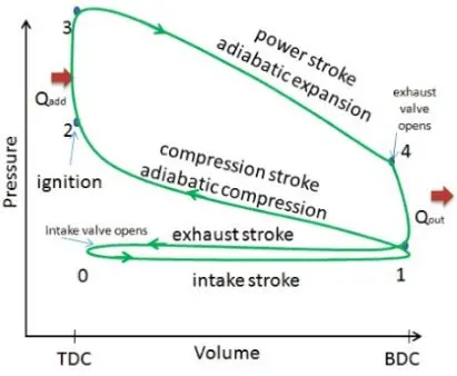
The otto cycle is an one of the air standard cycle, it is an idealized thermodynamic cycle that describes the function of a typical spark ignition piston engine. The Otto cycle is a description of what happens to a mass of gas as it is subjected to changes of pressure, temperature, volume, addition of heat, and removal of heat. The mass of gas that is subjected to those changes is called the system. The system, in this case, is defined to be the fluid (gas) within the cylinder.

Actual otto cycle pv diagram

Assumed otto cycle pv diagram

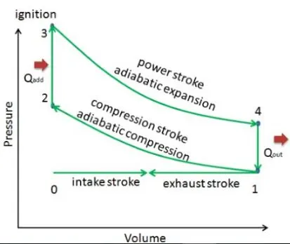
Assumption made for otto cycle

1) Working fluid is air, which continuously circulates in a closed loop cycle.

2) Air is considered as ideal gas.

3) Frictionless between piston and cylinder liner.

Thermodynamic processes

Process 0-1 : Constant Pressure air fuel mixture intake

Process 1-2 : Adiabatic or isentropic Compression process

Process 2-3 : Constant Volume heat addition

Process 3-4 : Adiabatic or isentropic expansion process

Process 4-1 :Constant Volume heat rejection

Process 1-0 : Constant pressure burn gas exhaust

GAS EQUATION

Adiabatic or isentropic process

`PV^gamma = Constant`

P - Pressure in pascals

V - Volume in meter^3

`gamma` - Ratio of specific heats = Cp/Cv = 1.4 for air, which is predominantly a diatomic gas

Ideal gas law

`(PV)/T = Constant`

P - Pressure

V - Volume

T - Temperature

Thermal efficiency

`eta = 1-(1/(cr)^(gamma-1))`

cr - Compression ratio

`eta` - Efficiency

`gamma` - ratio of specific heats

FORMULA FOR CALCULATING THE VOLUME CHANGE

`V = 1+1/2(cr-1)[R+1-costheta-(R^2-sin^2theta)^(1/2)]`

OBJECTIVE

1) To create a PV diagram for otto cycle and also calculate the thermal efficiency of an engine.

2) To visualize, how the thermodynamic properties values are change in each state point within the otto cycle.

3) To visualize the point function and path function.

4) Understanding the four stroke spark ignition engine within the otto cycle.

PYTHON PROGRAM :

"""
   Air Standard otto cycle
"""
import math                                                                      # Importing the math module for which calculating various trignometric function
import matplotlib.pyplot as plt                                                  # Importing the matplotlib, it's a plotting library


def engine_kinematics(bore, stroke, con_rod, Cr, start_crank, end_crank):        # Defining a function and it's name is engine_kinematics
	
	# Geometrical parameters
	a = stroke/2                                                                 # Crank pin radius, it distance between from crank axis to crank pin center axis
	R = con_rod/a                                                                # R is a constant, which is length of the connecting rod upon crank pin 

	# Volume parameters
	V_s = math.pi*(1/4)*pow(bore,2)*stroke                                       # Swept volume
	V_c = V_s/(Cr - 1)                                                           # Clearance volume
	sc = math.radians(start_crank)                                               # Convert the start crank in degree to radians
	ec = math.radians(end_crank)                                                 # Convert the end crank in degree to radians
	num_valve = 180                                                              # Number of values
	dtheta = (ec - sc)/(num_valve - 1)                                          

	V = []                                                                       # V Empty array                                 
   
	for i in range(0,num_valve):
		theta = sc + i*(dtheta)
		term1 = 0.5*(Cr - 1)
		term2 = R + 1 - math.cos(theta)
		term3 = pow(R,2) - pow(math.sin(theta),2)
		term3 = pow(term3,0.5)
		V.append((1 + term1*(term2 - term3))*V_c)
	return(V)

# Inputs
p1 = 101325
t1 = 500
t3 = 2000
gamma = 1.4

# Geometric parameters
bore = 0.1
stroke = 0.1
con_rod = 0.15
cr = 10

# Volume computation
v_s = (math.pi/4)*pow(bore,2)*stroke
v_c = v_s/(cr-1)
v1 = v_c + v_s

# State point 2
v2 = v_c

# p2v2^gamma = p1v1^gamma                                                             
p2 = p1*pow(v1,gamma)/pow(v2,gamma)

# p2v2/t2 = p1v1/t1 | rhs = p1v1/t1 | p2v2/t2 = rhs | t2 =p2v2/rhs                    
rhs = p1*v1/t1
t2 = p2*v2/rhs

V_compression = engine_kinematics (bore, stroke, con_rod, cr, 180, 0)               # Calling a function for which finding V_compressio
constant = p1*pow(v1,gamma)
P_compression = []

for v in V_compression:
	P_compression.append(constant/pow(v,gamma))

# State point 3
v3 = v2

# p3v3/t3 = p2v2/t2 | rhs = p2v2/t2 | p3 = rhs*t3/v3
rhs = p2*v2/t2
p3 = rhs*t3/v3

# State point 4
v4 = v1

#p4v4^gamma = p3v3^gamma 
p4 = p3*pow(v3,gamma)/pow(v4,gamma)

# p4v4/t4 = rhs
t4 = p4*v4/rhs

V_expansion = engine_kinematics (bore, stroke, con_rod, cr,0, 180)                   # Calling a function for which finding a V_expansion
constant = p3*pow(v3,gamma)
P_expansion = []

for V in V_expansion:
	P_expansion.append(constant/pow(V,gamma))

plt.plot([v2,v3],[p2,p3],label = 'Constant volume heat addition')
plt.plot(V_compression,P_compression,label = 'Isentropic compression process')
plt.plot(V_expansion,P_expansion,label = 'Isentropic expansion process')
plt.plot([v4,v1],[p4,p1],label = 'Constant volume heat rejection')
plt.xlabel('Volume in m^3')
plt.ylabel('Pressure in pascals')
plt.title('Air standard otto cycle)')
plt.legend()
plt.savefig('Otto Cycle')
plt.show() 

# Calculating a otto cycle thermal efficiency
efficiency = 1 - (1/pow(cr,gamma - 1))
print('Thermal Efficiency =')
print(efficiency)

EXPLANATION :

1) Importing the all needed modules like math & matplotlib. Math module is helps to calculating the various trigonometric ratio for as given angles, the function like sine, cosine, tangent, etc. In this case, we have put the angle in radians.

2) Providing the appropriate inputs such as pressure & temperature for state point 1 and temperature for state point 3. And also to providing the geometric parameters such as bore of the cylinder, stroke length of the cyclinder, length of the connecting rod and compression ratio of the cylinder.

3) Write a corresponding expression for calculating the swept volume and clearance volume.

4) By using isentropic or adiabatic expression and ideal gas law to calculate the otto cycle state point unknown thermodymaic properties such as p2, t2, v2, p3, v3, p4, v4, t4. Thus, it is a point function.

5) We want to trace out volume at where isentropic compression and expansion by which function of crank angle. We have one expression, it helps us to finding the volume trace at both compression and expansion.

6) Creating a function with defining the various variable such as bore, stroke, connecting rod length, compression ratio, starting crank angle and ending crank angle. A starting and ending crank angle is continuously varying in each and every ' for loop'.

7) We don't worry about constant heat addition and heat rejection.

8) Create a 'for loop' with range between from 0 to 180 , each iteration they give as to one value, that value either in Volume at compression or expansion.

9) By involve both volume variation at where compression and expansion into isentropic expansion. After that, we has also finding pressure at compression and expansion as well.

10) After all path function is calculated, we has plotted the air standard otto cycle by the help of matplotlib module. With that, we also finding thermal efficiency.

CODE SYNTAX EXPLAIN :

Math and matplotlib module is necessary to import at where top of the code. Math module is helps to calculating the various trignometric ratio for a given angle. A matplotlib module is help to create a plots. Corresponding snapshot is provided below

Defining the function with function name of engine kinematics and the function variable ar bore, stroke, connecting rod, compression ratio , strat crank & End crank. At the end the function, we have mandatory to put the colon symbol.

A geometric parameters, Volume parameters and for loops are under the function.

Create a 'for loop' in range between from 0 to 180.

A start and end values may exchange values it depends on calling a function.

In each 'for loop' value will appending into the empty V array, that value actually we use into volume compression as well as volume expansion. If we want to plot the isentropic compression curve, so we need put 180 at place of start crank, also put 0 at the place of end crank. If we want to plot the isentropic expansion curve, so we need put 0 instead of 180 at the place of start crank, also put 180 instead of 0 at the place of end crank.

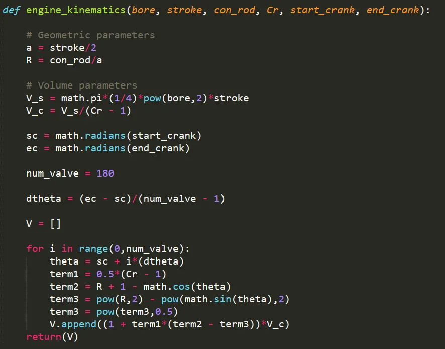
This is the calling function, order of the variables is same as defining function

RESULT AND DISCUSSION :

1) A blue colour curve indicates isentropic or adiabatic compression process, this process is happens at when the piston moves from BDC to TDC after the suction stroke. This stroke is called compression stroke.

2) A orange colour line indicates constant volume or Isochoric heat addition process, this process happens at after the compression stroke and also piston doesn't move. This stroke is called combustion stroke or power stroke.

3) A green colour curve indicates isentropic or adiabatic expansion process, this process is happens at when the piston moves to BDC from TDC after the combustion stroke. This stroke is called expansion stroke.

4) A red colour line indicates constant volume or Isochoric heat rejection process, this process happens at after the expansion stroke and also piston doesn't move from theoretically, but in practical piston should move.

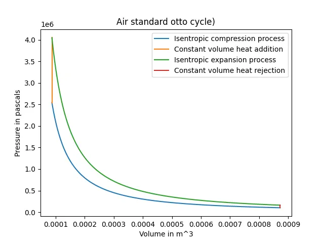
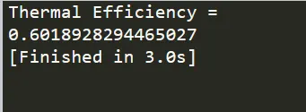
5) A thermal efficiency of the otto cycle in this case is 60.18 percent. Mainly, a efficiency varying depends on engine compression ratio.

CONCLUSION :

A successfully ran the python code and get the ouput of the air standard otto cycle and also finded the correspond thermal efficiency of the otto cycle.