Validation studies of Symmetry BC vs Wedge BC in OpenFOAM vs Analytical H.P equation
Aim:-
To simulate pipe flow using Wedge and Symmetry boundary conditions for different angles and validate them with the Hagen–Poiseuille equation.
Objective:-
- Validate Hydro-dynamic length with the numerical result
- Validate the fully developed flow velocity profile with its analytical profile
- Validate maximum velocity and pressured drop for fully developed flow
- Post-process Shear stress and validate wall shear stress for fully developed flow
- Highligh the differences in both boundary conditions in terms of their usage and application
This challenge is a continuation of a previous project, so we will directly dive into the simulation. The link to the previous project is given below where the introduction and the physics part are covered for your perusal.
https://skill-lync.com/student-projects/week-11-simulation-of-flow-through-a-pipe-in-openfoam-160
Methodology:-
In this project, we will be simulating the same case with different boundary conditions of Wedge and Symmetry for angles of 10, 25 and 45 respectively.
The Wedge boundary condition is used for 2-dimensional axisymmetric simulations, where the Navier-Stokes equations are taken in the Cylindrical co-ordinates. This boundary conditions yields an advantage of simulating a part of geometry with respect to its axis.
While the Symmetry boundary condition is used for the convenience of mirroring of the surface of the geometry which yields a decrease in the computational cost. The Symmetry boundary conditon takes the Navier-Stokes equations in Cartesian co-ordinates.
The workflow goes as follows:
- We will first generate our BlockMeshDict files with the Matlab code
- Then, run the simulations in OpenFoam
- Post-processing the data through analysing the resulting plots using Paraview
- And finally, validating the Numerical solutions with the Analytical solutions with the help of Matlab.
Input and Given parameters:
Pipe Data:
Diameter of the pipe `D =`0.0025 meters with Radius `R = D/2`
Reynold's Number `Re =`2100 (given)
Hydrodynaimc entry length `L_e = 0.05*Re*D`
Total length of the pipe `L = 0.3 + L_e`
Angle of the wedge `theta=3^o`
Fluid Data:
Type: Water at `20^o "Celsius"`
Density `rho = 997((kg)/m^3)`
Dynamic Viscosity `mu = 0.000890 ((N*s)/m^2)`
Kinematic Viscosity `nu = mu/rho`
Other calculated parameters:
Average velocity `V_(avg) = (Re*mu)/(rho*D)`
Maximum velocity `u_max = 2*V_(avg)`
Kinematic pressure `k_(p) = (Deltap)/rho`
Pre-Processing:-
The pre-processing part contains setting up the block mesh, boundary and initial conditions, physical properties and the simulation time. For the current simulation, we set up the mesh using BlockMeshDict file, the boundary and initial conditions using U, p files namely for velocity and pressure , physical properties using transportProperties file and the control (simulation parameters) using the ControlDict file.
The BlockMeshDict file is the most important and the primary step as it contains the block (mesh) parameters. To simplify editing the BlockMeshDict file, we have written a Matlab code which takes minimal parameters and yields the entire block mesh file. The Matlab code and the generated BlockMeshDict file is given below:
Matlab code:
clear all
close all
clc

% Input Data (meters)
D = 0.0025; % Diameter
R = D/2; % Radius
Re = 2100; % Reynolds Number
L_e = 0.05*Re*D; % Hydrodynamic Entry length
L = 0.3 + L_e; % Total Length
theta = 10; % Wedge Angle; Input the wedge angle here (10, 25, 45)

scale = 1; % All values referenced to 1 meter scale

% Vertices
v0 = [0 0 0];
v1 = [0 R*cosd(theta/2) -R*sind(theta/2)];
v2 = [0 R*cosd(theta/2) R*sind(theta/2)];
v3 = [L 0 0];
v4 = [L R*cosd(theta/2) -R*sind(theta/2)];
v5 = [L R*cosd(theta/2) R*sind(theta/2)];

% Block Parameters
cellx = 50; % Cells along x-axis
celly = 1; % Cells along y-axis
cellz = 400; % Cells along z-axis
gradx = 1; % Grading along x-axis
grady = 1; % Grading along y-axis
gradz = 1; % Grading along z-axis

% Arc inputs
arc1 = [1,2];
arc2 = [4,5];

f1 = fopen('BlockMeshDict.txt','w');
fprintf(f1,'%s\n','/*--------------------------------*- C++ -*----------------------------------*\');
fprintf(f1,'%s\n','  =========                 |');
fprintf(f1,'%s\n','  \\      /  F ield         | OpenFOAM: The Open Source CFD Toolbox');
fprintf(f1,'%s\n','   \\    /   O peration     | Website:  https://openfoam.org');
fprintf(f1,'%s\n','    \\  /    A nd           | Version:  6');
fprintf(f1,'%s\n','     \\/     M anipulation  |');
fprintf(f1,'%s\n','\*---------------------------------------------------------------------------*/');
fprintf(f1,'%s\n','FoamFile');
fprintf(f1,'%s\n','{');
fprintf(f1,'%s\n','    version     2.0;');
fprintf(f1,'%s\n','    format      ascii;');
fprintf(f1,'%s\n','    class       dictionary;');
fprintf(f1,'%s\n','    object      blockMeshDict;');
fprintf(f1,'%s\n','}');
fprintf(f1,'%s\n\n','// * * * * * * * * * * * * * * * * * * * * * * * * * * * * * * * * * * * * * //');
fprintf(f1,'%s %d;\n\n','convertToMeters',scale);

% Defining Vertices
fprintf(f1,'%s\n','vertices');
fprintf(f1,'%s\n','(');
fprintf(f1,'\t(%d %d %d)\n',v0(1),v0(2),v0(3));
fprintf(f1,'\t(%d %d %d)\n',v1(1),v1(2),v1(3));
fprintf(f1,'\t(%d %d %d)\n',v2(1),v2(2),v2(3));
fprintf(f1,'\t(%d %d %d)\n',v3(1),v3(2),v3(3));
fprintf(f1,'\t(%d %d %d)\n',v4(1),v4(2),v4(3));
fprintf(f1,'\t(%d %d %d)\n',v5(1),v5(2),v5(3));
fprintf(f1,'%s\n\n',');');

% Defining Blocks
fprintf(f1,'%s\n','blocks');
fprintf(f1,'%s\n','(');
fprintf(f1,'\thex (0 1 2 0 3 4 5 3)(%d %d %d) %s (%d %d %d)\n',cellx,celly,cellz,'simpleGrading',gradx,grady,gradz);
fprintf(f1,'%s\n\n',');');

% Defining Edges
fprintf(f1,'%s\n','edges');
fprintf(f1,'%s\n','(');
fprintf(f1,'\tarc %d %d (%d %d %d)\n',arc1(1),arc1(2),0,R,0);
fprintf(f1,'\tarc %d %d (%d %d %d)\n',arc2(1),arc2(2),L,R,0);
fprintf(f1,'%s\n',');');

% Defining Boundaries
fprintf(f1,'%s\n','boundary');
fprintf(f1,'%s\n','(');
fprintf(f1,'\tinlet\n\t{\n');
fprintf(f1,'\t\ttype patch;\n');
fprintf(f1,'\t\t faces \n\t\t(\n');
fprintf(f1,'\t\t\t(0 1 2 0)\n');
fprintf(f1,'\t\t);\n\t}\n');

fprintf(f1,'\toutlet\n\t{\n');
fprintf(f1,'\t\ttype patch;\n');
fprintf(f1,'\t\t faces \n\t\t(\n');
fprintf(f1,'\t\t\t(3 4 5 3)\n');
fprintf(f1,'\t\t);\n\t}\n');

fprintf(f1,'\tfront\n\t{\n');
fprintf(f1,'\t\ttype wedge;\n');
fprintf(f1,'\t\t faces \n\t\t(\n');
fprintf(f1,'\t\t\t(0 3 4 1)\n');
fprintf(f1,'\t\t);\n\t}\n');

fprintf(f1,'\tback\n\t{\n');
fprintf(f1,'\t\ttype wedge;\n');
fprintf(f1,'\t\t faces \n\t\t(\n');
fprintf(f1,'\t\t\t(0 3 5 2)\n');
fprintf(f1,'\t\t);\n\t}\n');

fprintf(f1,'\ttop\n\t{\n');
fprintf(f1,'\t\ttype wall;\n');
fprintf(f1,'\t\t faces \n\t\t(\n');
fprintf(f1,'\t\t\t(1 2 5 4)\n');
fprintf(f1,'\t\t);\n\t}\n');

fprintf(f1,'\taxis\n\t{\n');
fprintf(f1,'\t\ttype empty;\n');
fprintf(f1,'\t\t faces \n\t\t(\n');
fprintf(f1,'\t\t\t(0 3 3 0)\n');
fprintf(f1,'\t\t);\n\t}\n');
fprintf(f1,');\n\n');
fprintf(f1,'mergePatchPairs\n(\n);\n\n');
fprintf(f1,'// ************************************************************************* //');
fclose(f1);
BlockMeshDict:
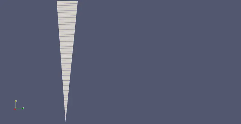
Wedge Case for `10^o`:
/*--------------------------------*- C++ -*----------------------------------*\
  =========                 |
  \\      /  F ield         | OpenFOAM: The Open Source CFD Toolbox
   \\    /   O peration     | Website:  https://openfoam.org
    \\  /    A nd           | Version:  6
     \\/     M anipulation  |
\*---------------------------------------------------------------------------*/
FoamFile
{
    version     2.0;
    format      ascii;
    class       dictionary;
    object      blockMeshDict;
}
// * * * * * * * * * * * * * * * * * * * * * * * * * * * * * * * * * * * * * //

convertToMeters 1;

vertices
(
	(0 0 0)
	(0 1.245243e-03 -1.089447e-04)
	(0 1.245243e-03 1.089447e-04)
	(5.625000e-01 0 0)
	(5.625000e-01 1.245243e-03 -1.089447e-04)
	(5.625000e-01 1.245243e-03 1.089447e-04)
);

blocks
(
	hex (0 1 2 0 3 4 5 3)(50 1 400) simpleGrading (1 1 1)
);

edges
(
	arc 1 2 (0 1.250000e-03 0)
	arc 4 5 (5.625000e-01 1.250000e-03 0)
);
boundary
(
	inlet
	{
		type patch;
		 faces
		(
			(0 1 2 0)
		);
	}
	outlet
	{
		type patch;
		 faces
		(
			(3 4 5 3)
		);
	}
	front
	{
		type wedge;
		 faces
		(
			(0 3 4 1)
		);
	}
	back
	{
		type wedge;
		 faces
		(
			(0 3 5 2)
		);
	}
	top
	{
		type wall;
		 faces
		(
			(1 2 5 4)
		);
	}
	axis
	{
		type empty;
		 faces
		(
			(0 3 3 0)
		);
	}
);

mergePatchPairs
(
);

// ************************************************************************* //
Snapshot of generated mesh:
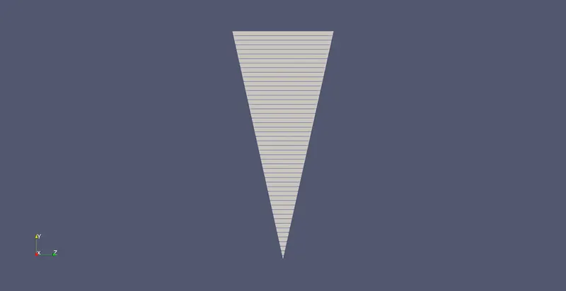
Wedge Case for `25^o`:
/*--------------------------------*- C++ -*----------------------------------*\
  =========                 |
  \\      /  F ield         | OpenFOAM: The Open Source CFD Toolbox
   \\    /   O peration     | Website:  https://openfoam.org
    \\  /    A nd           | Version:  6
     \\/     M anipulation  |
\*---------------------------------------------------------------------------*/
FoamFile
{
    version     2.0;
    format      ascii;
    class       dictionary;
    object      blockMeshDict;
}
// * * * * * * * * * * * * * * * * * * * * * * * * * * * * * * * * * * * * * //

convertToMeters 1;

vertices
(
	(0 0 0)
	(0 1.220370e-03 -2.705495e-04)
	(0 1.220370e-03 2.705495e-04)
	(5.625000e-01 0 0)
	(5.625000e-01 1.220370e-03 -2.705495e-04)
	(5.625000e-01 1.220370e-03 2.705495e-04)
);

blocks
(
	hex (0 1 2 0 3 4 5 3)(50 1 400) simpleGrading (1 1 1)
);

edges
(
	arc 1 2 (0 1.250000e-03 0)
	arc 4 5 (5.625000e-01 1.250000e-03 0)
);
boundary
(
	inlet
	{
		type patch;
		 faces
		(
			(0 1 2 0)
		);
	}
	outlet
	{
		type patch;
		 faces
		(
			(3 4 5 3)
		);
	}
	front
	{
		type wedge;
		 faces
		(
			(0 3 4 1)
		);
	}
	back
	{
		type wedge;
		 faces
		(
			(0 3 5 2)
		);
	}
	top
	{
		type wall;
		 faces
		(
			(1 2 5 4)
		);
	}
	axis
	{
		type empty;
		 faces
		(
			(0 3 3 0)
		);
	}
);

mergePatchPairs
(
);

// ************************************************************************* //
Snapshot of generated mesh:
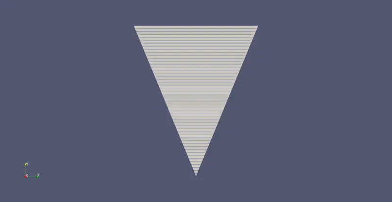
Wedge Case for `45^o`:
/*--------------------------------*- C++ -*----------------------------------*\
  =========                 |
  \\      /  F ield         | OpenFOAM: The Open Source CFD Toolbox
   \\    /   O peration     | Website:  https://openfoam.org
    \\  /    A nd           | Version:  6
     \\/     M anipulation  |
\*---------------------------------------------------------------------------*/
FoamFile
{
    version     2.0;
    format      ascii;
    class       dictionary;
    object      blockMeshDict;
}
// * * * * * * * * * * * * * * * * * * * * * * * * * * * * * * * * * * * * * //

convertToMeters 1;

vertices
(
	(0 0 0)
	(0 1.154849e-03 -4.783543e-04)
	(0 1.154849e-03 4.783543e-04)
	(5.625000e-01 0 0)
	(5.625000e-01 1.154849e-03 -4.783543e-04)
	(5.625000e-01 1.154849e-03 4.783543e-04)
);

blocks
(
	hex (0 1 2 0 3 4 5 3)(50 1 400) simpleGrading (1 1 1)
);

edges
(
	arc 1 2 (0 1.250000e-03 0)
	arc 4 5 (5.625000e-01 1.250000e-03 0)
);
boundary
(
	inlet
	{
		type patch;
		 faces
		(
			(0 1 2 0)
		);
	}
	outlet
	{
		type patch;
		 faces
		(
			(3 4 5 3)
		);
	}
	front
	{
		type wedge;
		 faces
		(
			(0 3 4 1)
		);
	}
	back
	{
		type wedge;
		 faces
		(
			(0 3 5 2)
		);
	}
	top
	{
		type wall;
		 faces
		(
			(1 2 5 4)
		);
	}
	axis
	{
		type empty;
		 faces
		(
			(0 3 3 0)
		);
	}
);

mergePatchPairs
(
);

// ************************************************************************* //
Snapshot of generated mesh:
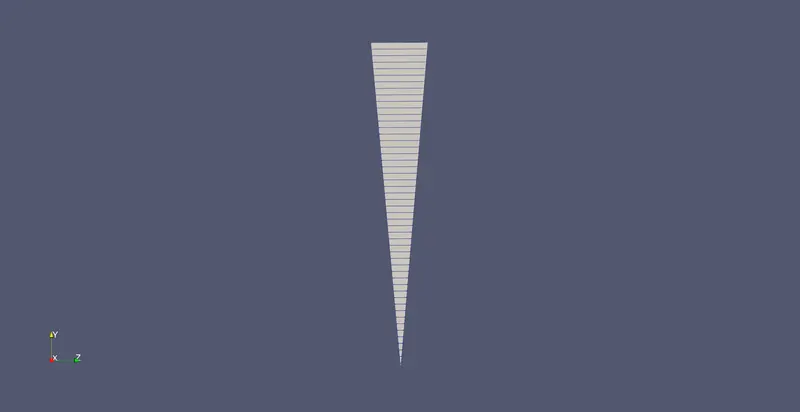
Symmetry Case for `10^o`:
/*--------------------------------*- C++ -*----------------------------------*\
  =========                 |
  \\      /  F ield         | OpenFOAM: The Open Source CFD Toolbox
   \\    /   O peration     | Website:  https://openfoam.org
    \\  /    A nd           | Version:  6
     \\/     M anipulation  |
\*---------------------------------------------------------------------------*/
FoamFile
{
    version     2.0;
    format      ascii;
    class       dictionary;
    object      blockMeshDict;
}
// * * * * * * * * * * * * * * * * * * * * * * * * * * * * * * * * * * * * * //

convertToMeters 1;

vertices
(
	(0 0 0)
	(0 1.245243e-03 -1.089447e-04)
	(0 1.245243e-03 1.089447e-04)
	(5.625000e-01 0 0)
	(5.625000e-01 1.245243e-03 -1.089447e-04)
	(5.625000e-01 1.245243e-03 1.089447e-04)
);

blocks
(
	hex (0 1 2 0 3 4 5 3)(50 1 400) simpleGrading (1 1 1)
);

edges
(
	arc 1 2 (0 1.250000e-03 0)
	arc 4 5 (5.625000e-01 1.250000e-03 0)
);
boundary
(
	inlet
	{
		type patch;
		 faces
		(
			(0 1 2 0)
		);
	}
	outlet
	{
		type patch;
		 faces
		(
			(3 4 5 3)
		);
	}
	front
	{
		type symmetry;
		 faces
		(
			(0 3 4 1)
		);
	}
	back
	{
		type symmetry;
		 faces
		(
			(0 3 5 2)
		);
	}
	top
	{
		type wall;
		 faces
		(
			(1 2 5 4)
		);
	}
	axis
	{
		type empty;
		 faces
		(
			(0 3 3 0)
		);
	}
);

mergePatchPairs
(
);

// ************************************************************************* //
Snapshot of generated mesh:
Symmetry Case for `25^o`:
/*--------------------------------*- C++ -*----------------------------------*\
  =========                 |
  \\      /  F ield         | OpenFOAM: The Open Source CFD Toolbox
   \\    /   O peration     | Website:  https://openfoam.org
    \\  /    A nd           | Version:  6
     \\/     M anipulation  |
\*---------------------------------------------------------------------------*/
FoamFile
{
    version     2.0;
    format      ascii;
    class       dictionary;
    object      blockMeshDict;
}
// * * * * * * * * * * * * * * * * * * * * * * * * * * * * * * * * * * * * * //

convertToMeters 1;

vertices
(
	(0 0 0)
	(0 1.220370e-03 -2.705495e-04)
	(0 1.220370e-03 2.705495e-04)
	(5.625000e-01 0 0)
	(5.625000e-01 1.220370e-03 -2.705495e-04)
	(5.625000e-01 1.220370e-03 2.705495e-04)
);

blocks
(
	hex (0 1 2 0 3 4 5 3)(50 1 400) simpleGrading (1 1 1)
);

edges
(
	arc 1 2 (0 1.250000e-03 0)
	arc 4 5 (5.625000e-01 1.250000e-03 0)
);
boundary
(
	inlet
	{
		type patch;
		 faces
		(
			(0 1 2 0)
		);
	}
	outlet
	{
		type patch;
		 faces
		(
			(3 4 5 3)
		);
	}
	front
	{
		type symmetry;
		 faces
		(
			(0 3 4 1)
		);
	}
	back
	{
		type symmetry;
		 faces
		(
			(0 3 5 2)
		);
	}
	top
	{
		type wall;
		 faces
		(
			(1 2 5 4)
		);
	}
	axis
	{
		type empty;
		 faces
		(
			(0 3 3 0)
		);
	}
);

mergePatchPairs
(
);

// ************************************************************************* //
Snapshot of generated mesh:
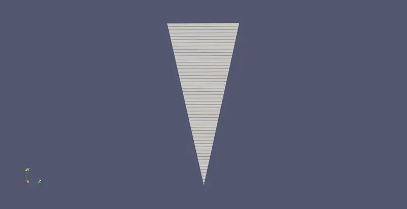
Symmetry Case for `45^o`:
/*--------------------------------*- C++ -*----------------------------------*\
  =========                 |
  \\      /  F ield         | OpenFOAM: The Open Source CFD Toolbox
   \\    /   O peration     | Website:  https://openfoam.org
    \\  /    A nd           | Version:  6
     \\/     M anipulation  |
\*---------------------------------------------------------------------------*/
FoamFile
{
    version     2.0;
    format      ascii;
    class       dictionary;
    object      blockMeshDict;
}
// * * * * * * * * * * * * * * * * * * * * * * * * * * * * * * * * * * * * * //

convertToMeters 1;

vertices
(
	(0 0 0)
	(0 1.154849e-03 -4.783543e-04)
	(0 1.154849e-03 4.783543e-04)
	(5.625000e-01 0 0)
	(5.625000e-01 1.154849e-03 -4.783543e-04)
	(5.625000e-01 1.154849e-03 4.783543e-04)
);

blocks
(
	hex (0 1 2 0 3 4 5 3)(50 1 400) simpleGrading (1 1 1)
);

edges
(
	arc 1 2 (0 1.250000e-03 0)
	arc 4 5 (5.625000e-01 1.250000e-03 0)
);
boundary
(
	inlet
	{
		type patch;
		 faces
		(
			(0 1 2 0)
		);
	}
	outlet
	{
		type patch;
		 faces
		(
			(3 4 5 3)
		);
	}
	front
	{
		type symmetry;
		 faces
		(
			(0 3 4 1)
		);
	}
	back
	{
		type symmetry;
		 faces
		(
			(0 3 5 2)
		);
	}
	top
	{
		type wall;
		 faces
		(
			(1 2 5 4)
		);
	}
	axis
	{
		type empty;
		 faces
		(
			(0 3 3 0)
		);
	}
);

mergePatchPairs
(
);

// ************************************************************************* //
Snapshot of generated mesh:
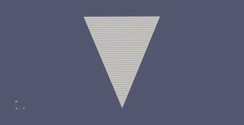
U file:
The U file is located in the '0' folder and is used for specifying the inlet and boundary conditions for velocity. Here, we have given inlet as uniform and a value of 0.7498 m/sec which is fixed in the x-direction. The outlet is specified as zeroGradient which is a Neumann Boundary condition as we have a pressure outlet and we will calculate the velocity at the outlet as part of the time marching simulation. Moving on, the front and back are specified as wedge boundary condition. For the Symmetry boundary condition, we replace the wedge part for front and back with symmetry. The top (wall) is specified with noSlip conditon. The pipe wall imparts a large shear stress onto the fluid particles that are in contact with it causing them to have zero velocity, this is called the noSlip condition. Finally, the axis specified as empty to regulate the calculation of fluid characteristics at the axis domain.
/*--------------------------------*- C++ -*----------------------------------*\
  =========                 |
  \\      /  F ield         | OpenFOAM: The Open Source CFD Toolbox
   \\    /   O peration     | Website:  https://openfoam.org
    \\  /    A nd           | Version:  6
     \\/     M anipulation  |
\*---------------------------------------------------------------------------*/
FoamFile
{
    version     2.0;
    format      ascii;
    class       volVectorField;
    object      U;
}
// * * * * * * * * * * * * * * * * * * * * * * * * * * * * * * * * * * * * * //

dimensions      [0 1 -1 0 0 0 0];

internalField   uniform (0.07498 0 0);

boundaryField
{
    inlet
    {
        type            fixedValue;
        value           uniform (0.07498 0 0);
    }

    outlet
    {
        type            zeroGradient;
    }

    front
    {
        type            wedge;
    }

    back
    {
        type            wedge;
    }

    top
    {
        type            fixedValue;
        value           uniform (0 0 0);
    }

    axis
    {
        type            empty;
    }
}

// ************************************************************************* //
For Symmetry Boundary Condition:
/*--------------------------------*- C++ -*----------------------------------*\
  =========                 |
  \\      /  F ield         | OpenFOAM: The Open Source CFD Toolbox
   \\    /   O peration     | Website:  https://openfoam.org
    \\  /    A nd           | Version:  8
     \\/     M anipulation  |
\*---------------------------------------------------------------------------*/
FoamFile
{
    version     2.0;
    format      ascii;
    class       volVectorField;
    object      U;
}
// * * * * * * * * * * * * * * * * * * * * * * * * * * * * * * * * * * * * * //

dimensions      [0 1 -1 0 0 0 0];

internalField   uniform (0.7498 0 0);

boundaryField
{

    inlet
    {
        type            fixedValue;
		value			uniform (0.7498 0 0);
    }

    outlet
    {
        type            zeroGradient;
    }

    front
    {
        type            symmetry;
    }

    back
    {
        type            symmetry;
    }

    top
    {
        type            noSlip;
    }

    axis
    {
        type            empty;
    }
}

// ************************************************************************* //
P file:
This file is also located in the '0' folder and is used for specifying the inlet and boundary conditions for pressure. The inlet is given as zeroGradient which is a Neumann Boundary Condition and will be calculated during the time marching part of the simulation. The outlet is a fixed value and specified as uniform 0 indicating the guage pressure which is related to the atmospheric pressure in this case 1 atm. Similar to the U file, front and back are specified as wedge boundary conditions and axis as empty to regulate the calculation of fluid characteristics at the axis domain. top is specified as zeroGradient as it will be calculated during the time marching part of the simulation.
/*--------------------------------*- C++ -*----------------------------------*\
  =========                 |
  \\      /  F ield         | OpenFOAM: The Open Source CFD Toolbox
   \\    /   O peration     | Website:  https://openfoam.org
    \\  /    A nd           | Version:  6
     \\/     M anipulation  |
\*---------------------------------------------------------------------------*/
FoamFile
{
    version     2.0;
    format      ascii;
    class       volScalarField;
    object      p;
}
// * * * * * * * * * * * * * * * * * * * * * * * * * * * * * * * * * * * * * //

dimensions      [0 2 -2 0 0 0 0];

internalField   uniform 0;

boundaryField
{
    inlet
    {
        type            zeroGradient;
    }

    outlet
    {
        type            fixedValue;
        value           uniform 0;
    }

    front
    {
        type            wedge;
    }

    back
    {
        type            wedge;
    }

    top
    {
        type            zeroGradient;
    }

    axis
    {
        type            empty;
    }
}

// ************************************************************************* //
For Symmetry Boundary Condition:
/*--------------------------------*- C++ -*----------------------------------*\
  =========                 |
  \\      /  F ield         | OpenFOAM: The Open Source CFD Toolbox
   \\    /   O peration     | Website:  https://openfoam.org
    \\  /    A nd           | Version:  8
     \\/     M anipulation  |
\*---------------------------------------------------------------------------*/
FoamFile
{
    version     2.0;
    format      ascii;
    class       volScalarField;
    object      p;
}
// * * * * * * * * * * * * * * * * * * * * * * * * * * * * * * * * * * * * * //

dimensions      [0 2 -2 0 0 0 0];

internalField   uniform 0;

boundaryField
{
	inlet
    {
        type            zeroGradient;
    }

    outlet
    {
        type            fixedValue;
		value			uniform 0;
    }

    front
    {
        type            symmetry;
    }

    back
    {
        type            symmetry;
    }

    top
    {
        type            zeroGradient;
    }

    axis
    {
        type            empty;
    }
}

// ************************************************************************* //
Note:
While setting up the BlockMeshDict, U and p files, it is very important to maintain same boundary parameters (inlet, outlet, front, etc..), if not OpenFoam throws an error called "cannot find patchfield entry" due to mismatched parameters.
ControlDict:
The OpenFOAM solvers begin all runs by setting up a database that controls Input/Output and, since output of data is usually requested at intervals of time during the simualtion run, as time is an inextricable part of the database. The controlDict dictionary stands for time and data Input/Output control and sets the I/O parameters for the creation of the database. This dictionary contains the start, end time for the simulation including the time step size. Here, we have given end time of 5 with time step of 0.001, so we have about 5000 iterations. It also contains a parameter called writeInterval at which data is saved into the solution database which means it will take data for every 50 iterations. These parameters are mandatory and have default values stored in sample cases which can be tweaked according to the user's specification and the nature of the simulation.
/*--------------------------------*- C++ -*----------------------------------*\
  =========                 |
  \\      /  F ield         | OpenFOAM: The Open Source CFD Toolbox
   \\    /   O peration     | Website:  https://openfoam.org
    \\  /    A nd           | Version:  8
     \\/     M anipulation  |
\*---------------------------------------------------------------------------*/
FoamFile
{
    version     2.0;
    format      ascii;
    class       dictionary;
    location    "system";
    object      controlDict;
}
// * * * * * * * * * * * * * * * * * * * * * * * * * * * * * * * * * * * * * //

application     icoFoam;

startFrom       startTime;

startTime       0;

stopAt          endTime;

endTime         5;

deltaT          1e-3;

writeControl    timeStep;

writeInterval   50;

purgeWrite      0;

writeFormat     ascii;

writePrecision  6;

writeCompression off;

timeFormat      general;

timePrecision   6;

runTimeModifiable true;


// ************************************************************************* //
transportProperties:
In OpenFoam, solvers which do not include energy/heat parameters, include libraries of models for viscosity `(nu)`. These models generally relate viscosity to strain rate `(dot gamma)` and are specified by the user in the transportProperties dictionary.
/*--------------------------------*- C++ -*----------------------------------*\
  =========                 |
  \\      /  F ield         | OpenFOAM: The Open Source CFD Toolbox
   \\    /   O peration     | Website:  https://openfoam.org
    \\  /    A nd           | Version:  8
     \\/     M anipulation  |
\*---------------------------------------------------------------------------*/
FoamFile
{
    version     2.0;
    format      ascii;
    class       dictionary;
    location    "constant";
    object      transportProperties;
}
// * * * * * * * * * * * * * * * * * * * * * * * * * * * * * * * * * * * * * //

nu              [0 2 -1 0 0 0 0] 8.92e-07;


// ************************************************************************* //
At this point, we are done with the pre-processing part of this project. To run the simulation, we use the 'icoFoam' command to invoke the icofoam solver which is an incompressible laminar Navier-Stokes equation solver using the PISO algorithm. The simulation will start and the residuals are displayed accordingly and will run as specified in the controlDict file until the residuals converge. After the simulation is done, we step into the post-processing phase of our project.
Post-Processing:
Velocity Distribution at pipe entrance
Velocity Distribution at pipe exit
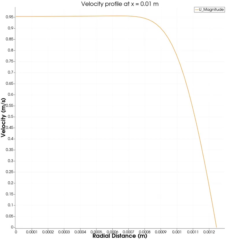
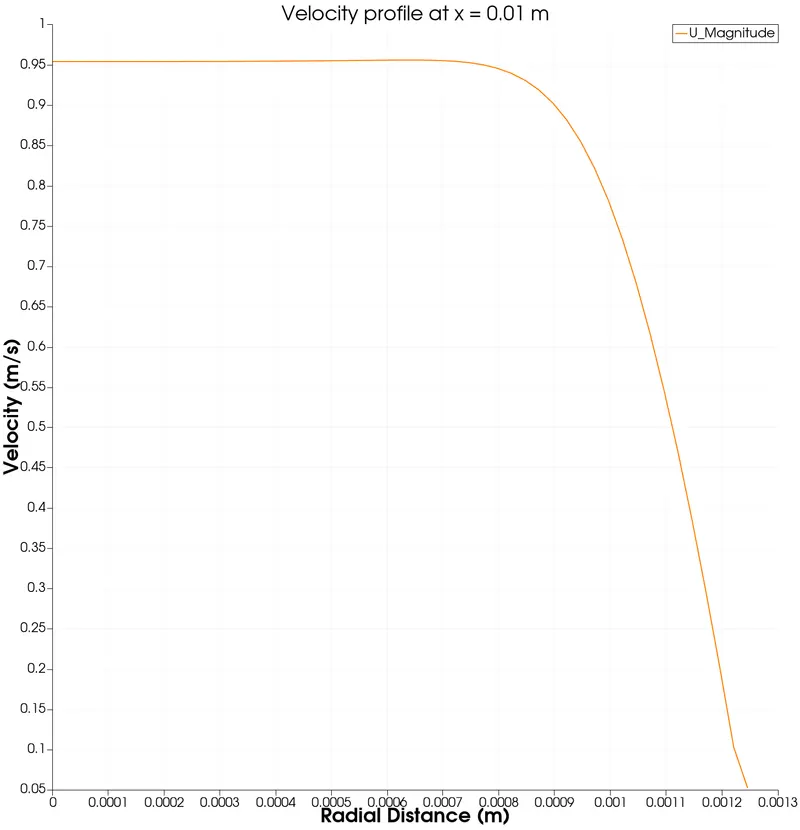
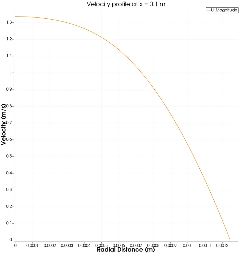
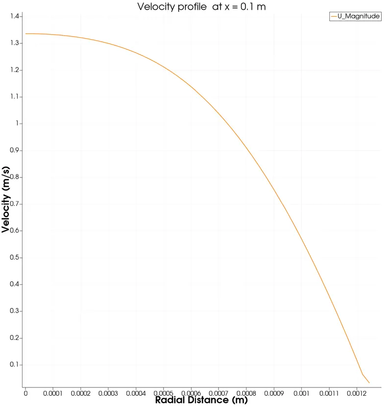
Velocity profiles: -
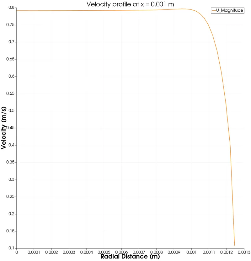
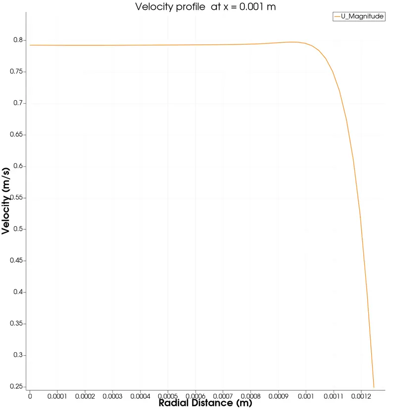
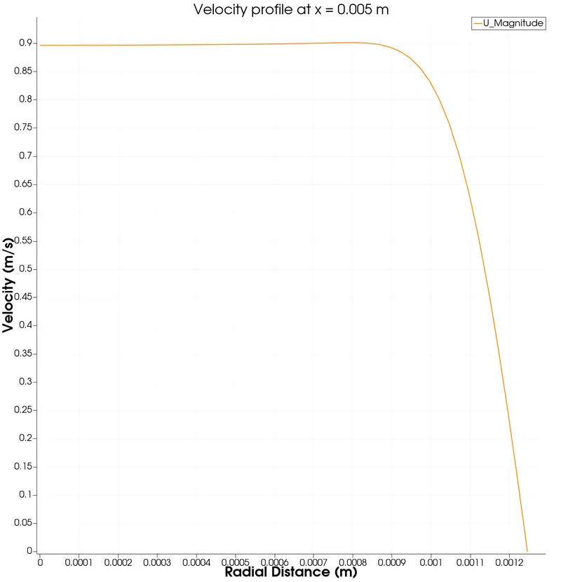
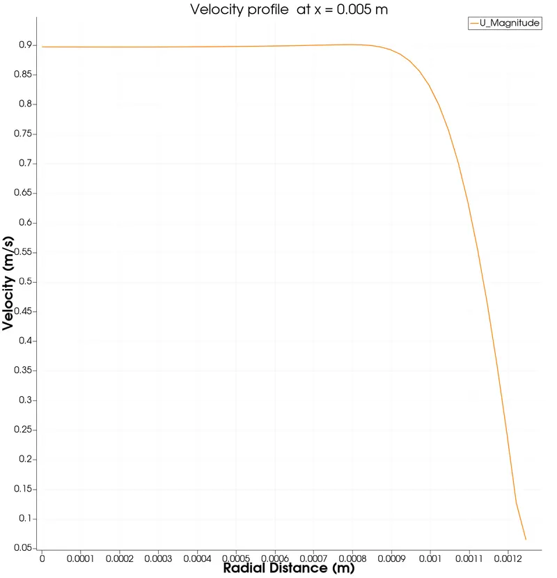
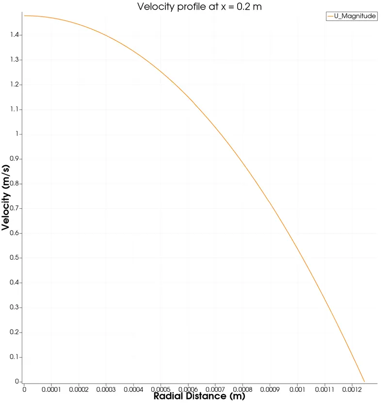
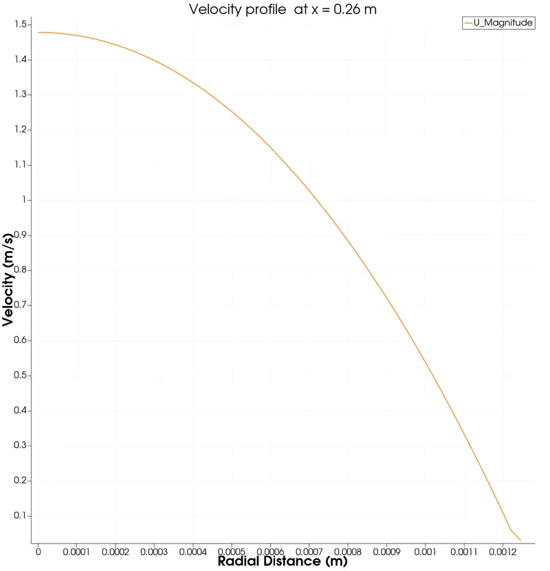
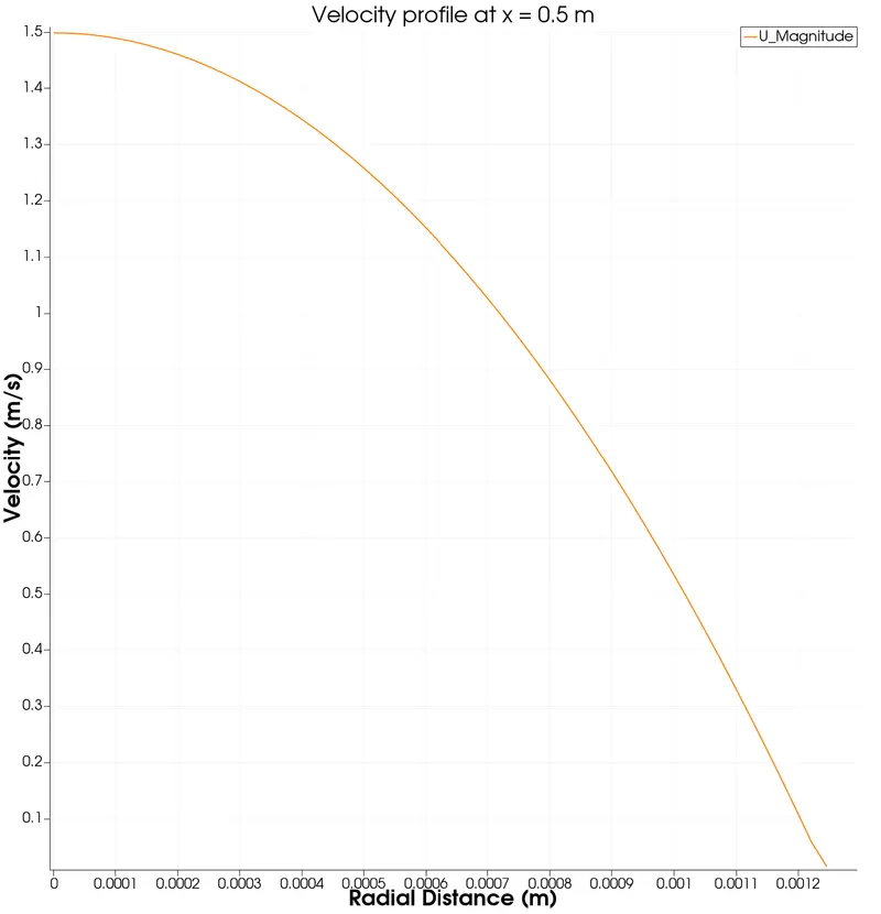
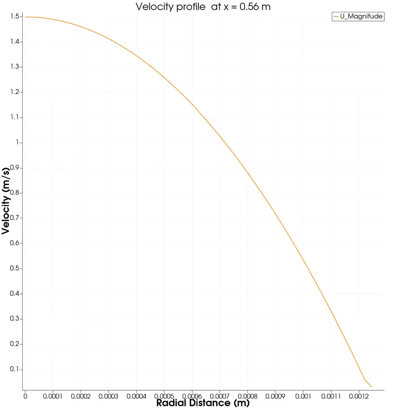
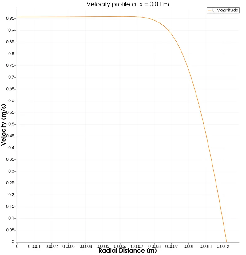
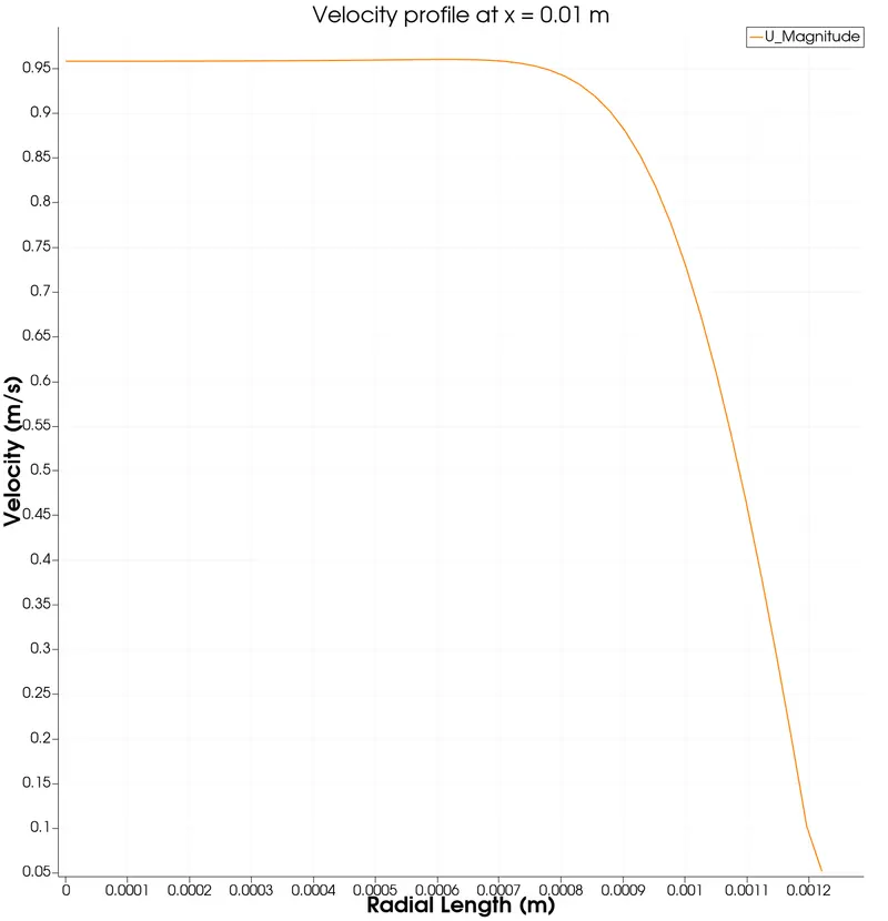
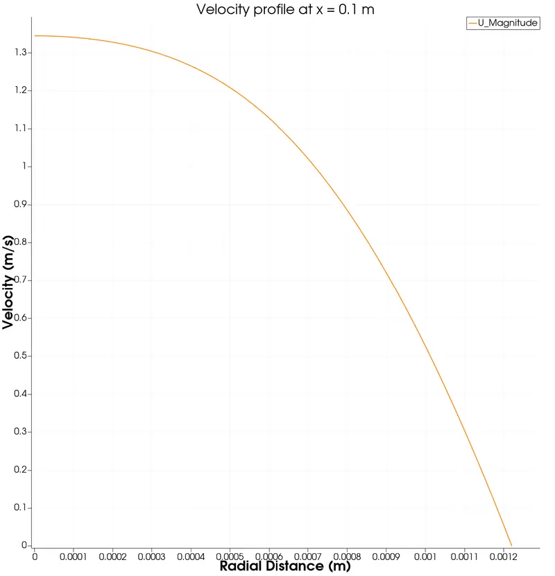
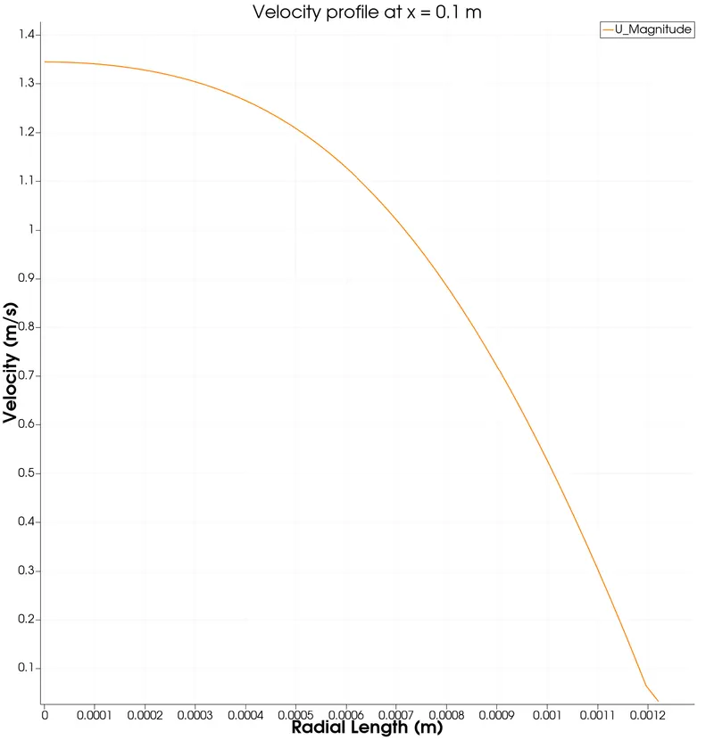
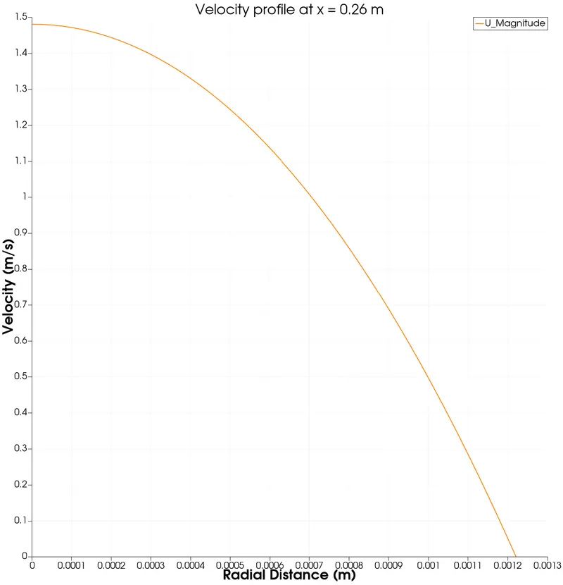
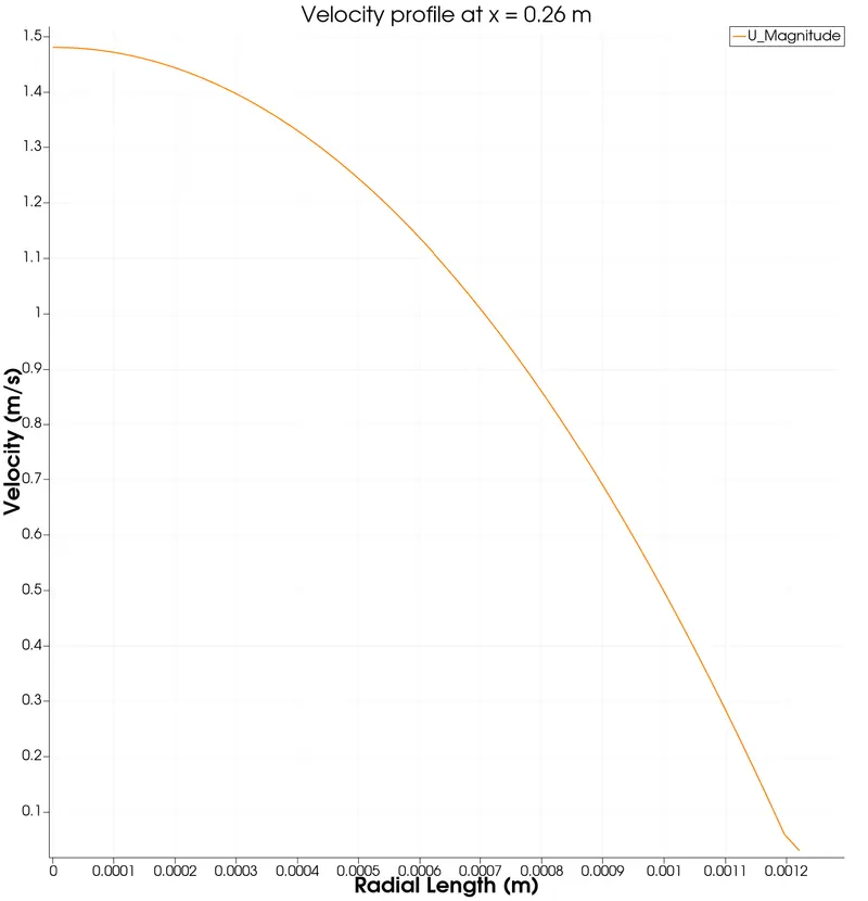
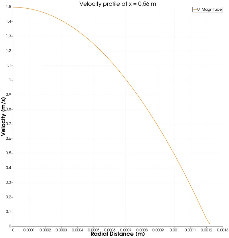
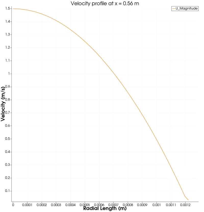
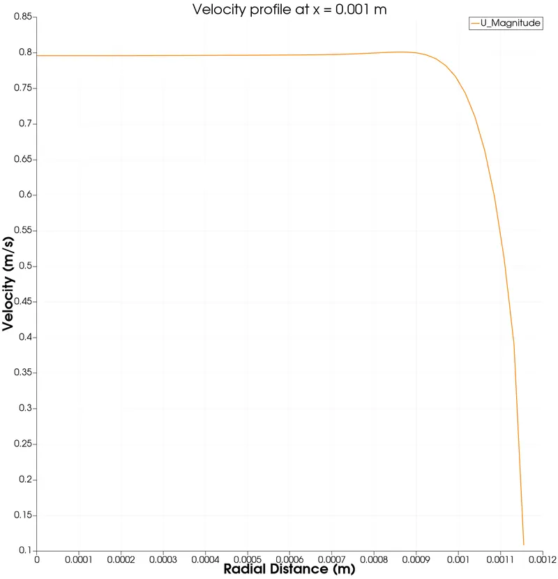
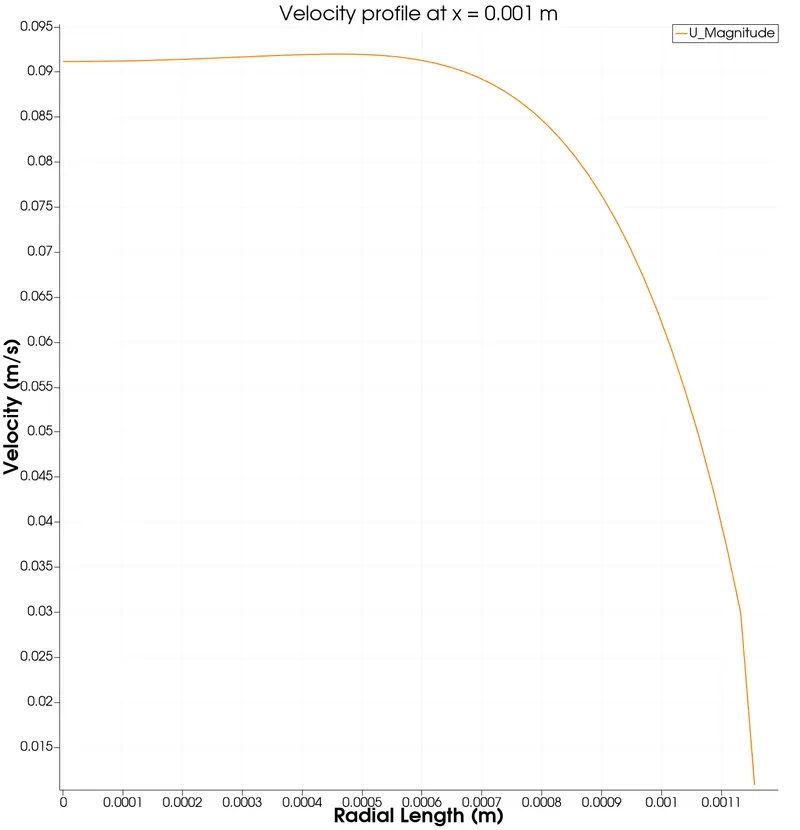
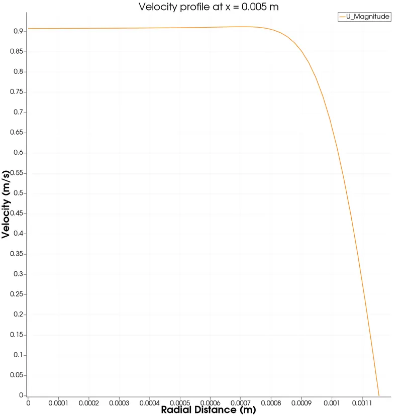
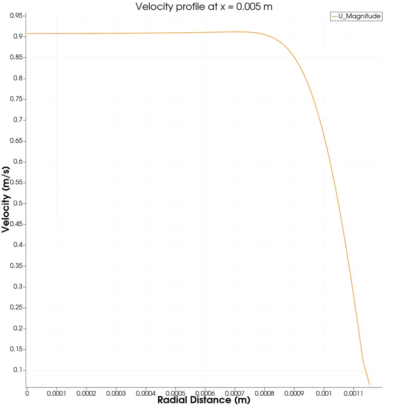
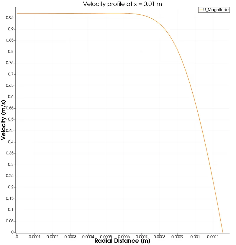
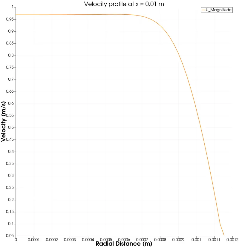
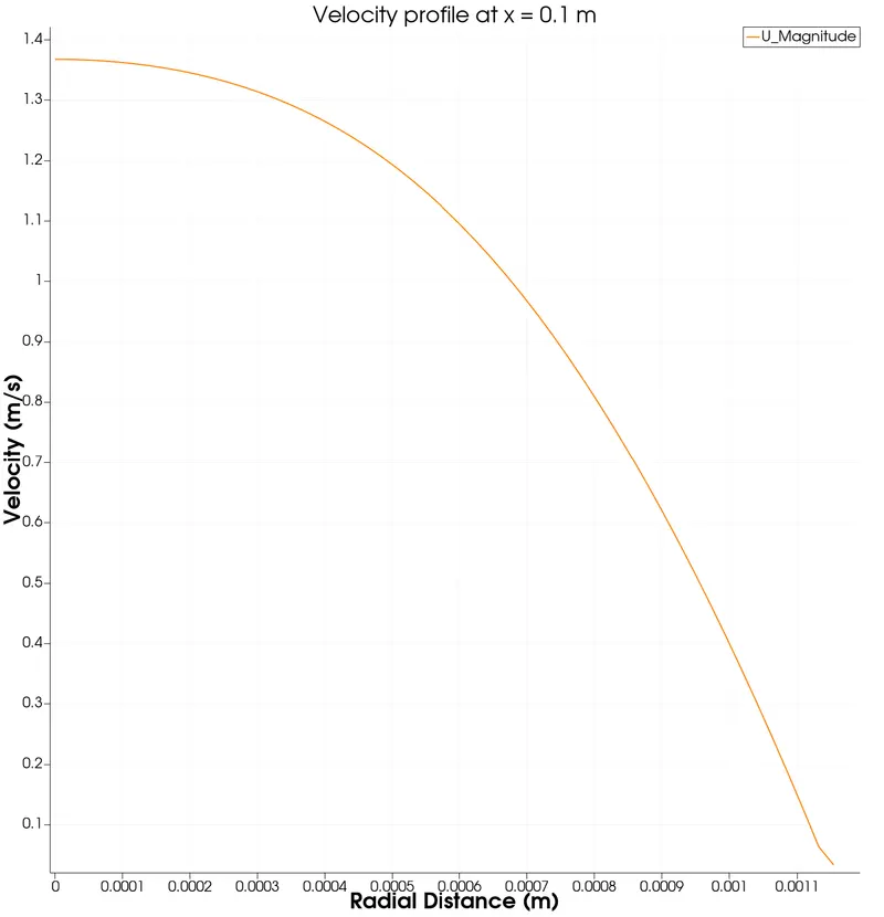
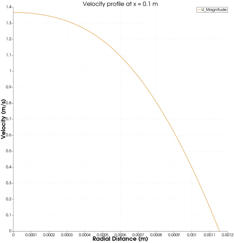
We will now be plotting the velocity profile at different locations of the x domain to understand how the flow is gradually formed.
Wedge Symmetry
`10^o`:
At distance 0.001 m from inlet
At distance 0.005 m from inlet
At distance 0.01 m from inlet
At distance 0.1 m from inlet
At distance 0.2 m from inlet
At distance 0.5 m from inlet
`25^o`:
At distance 0.001 m from inlet
At distance 0.005 m from inlet
At distance 0.01 m from inlet
At distance 0.1 m from inlet
At distance 0.2 m from inlet
At distance 0.5 m from inlet
`45^o`:
At distance 0.001 m from inlet
At distance 0.005 m from inlet
At distance 0.01 m from inlet
At distance 0.1 m from inlet
At distance 0.2 m from inlet
At distance 0.5 m from inlet
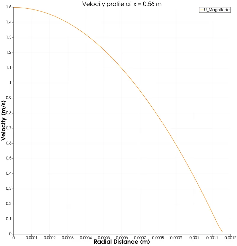
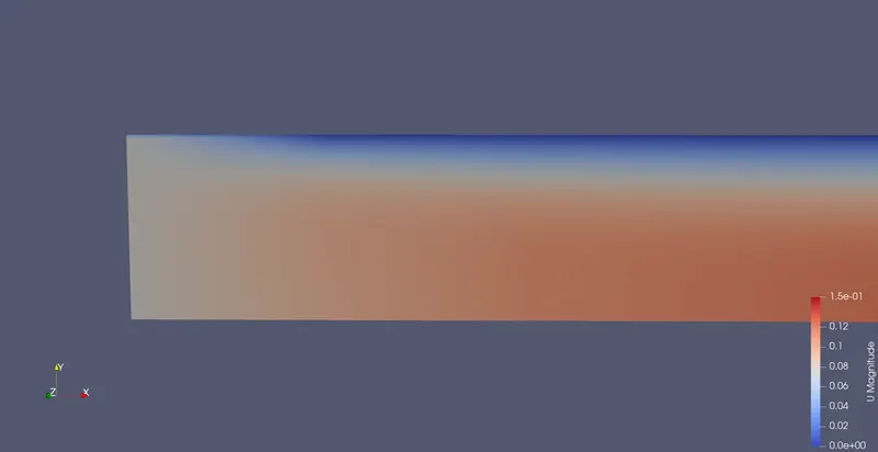
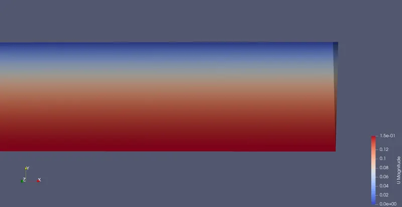
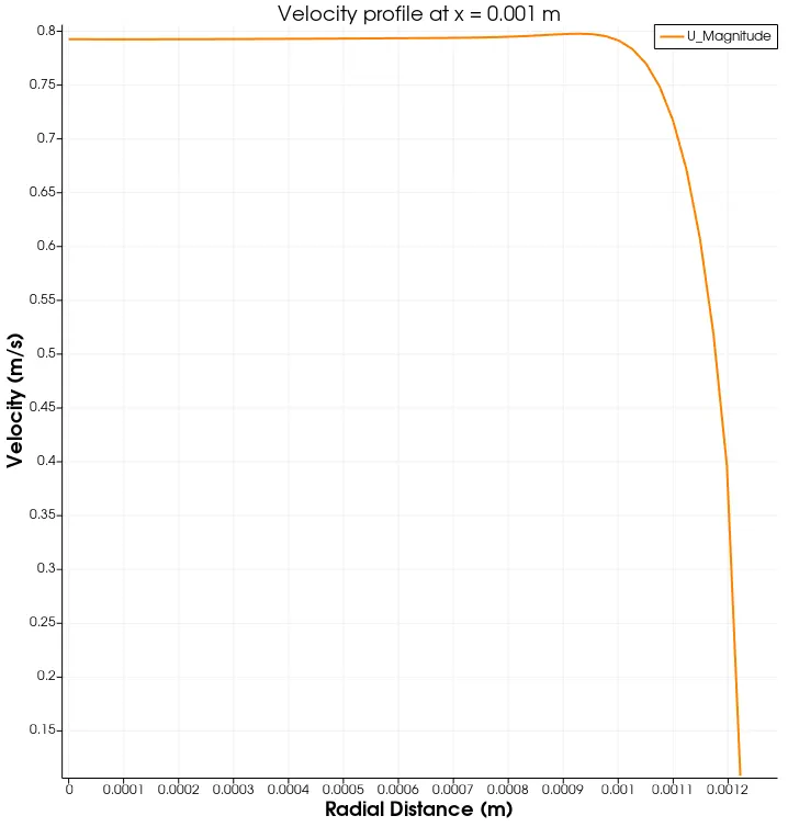
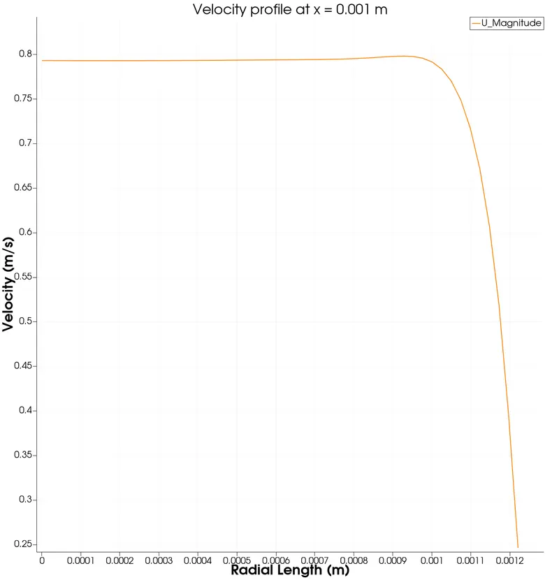
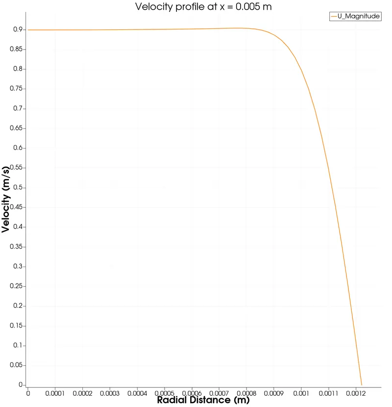
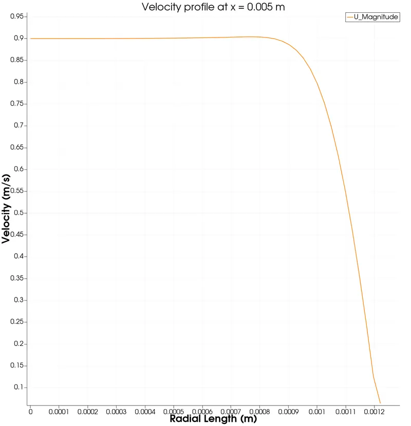
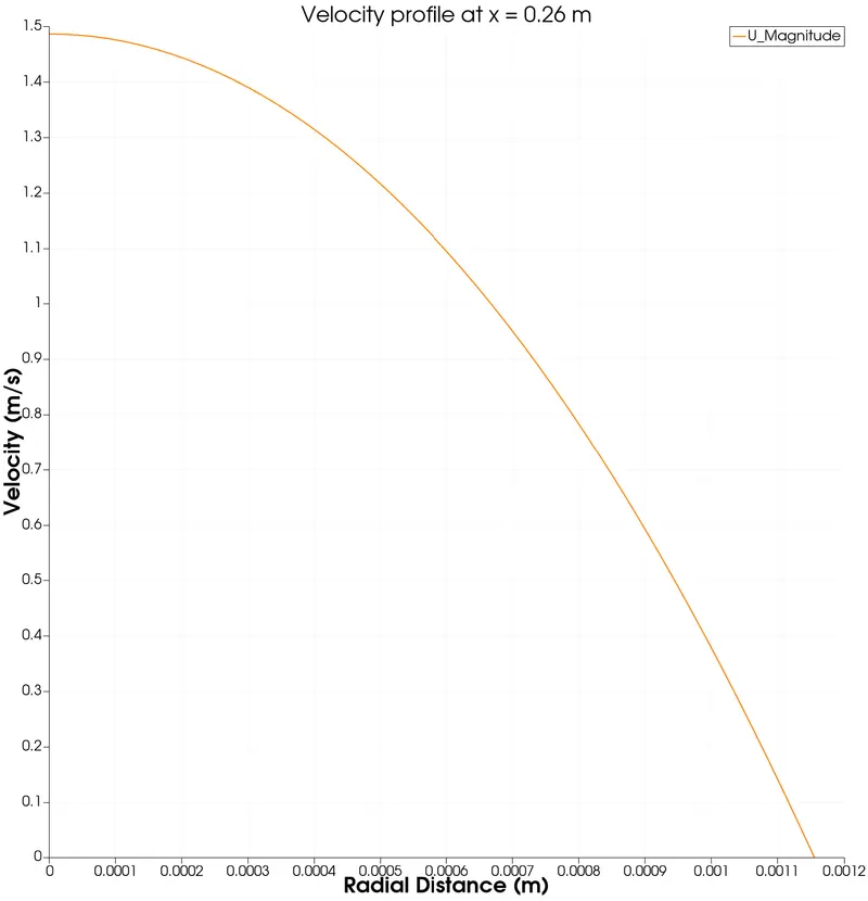
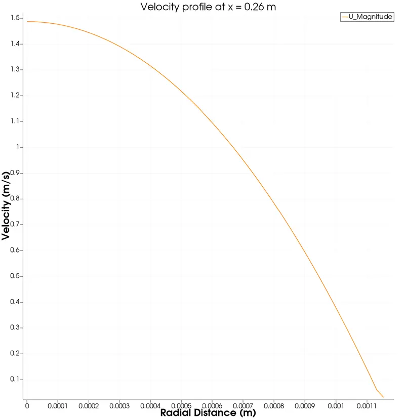
The velocity profiles seen above for Wedge and Symmetry bounary conditions for `10^o, 25^o` and `45^o` are very similar. From the above plots, we can see how the velocity profile is developing in the hydrodynamic entry region (0.2625 m) and at the fully developed region (0.5625 m) for all the respective cases. We see that there is a development in the velocity profile up until the hydeodynamic entrance length for all the cases. From there, we enter the fully developed flow region where the velocity settles to a constant value. For the hydeodynamic entrance length velocity profiles, we see that velocity is slowly increasing and then going to a stangnant value, this is because we are plotting the line of the plot from the axis to the wall. The velocity has a 0 value at the wall due to the shear stress imparted there due to the no slip condition. While near the axis, the shear stress is very neglgilble and the velocity is at its maximum. This maximum velocity is almost same for all the cases with negligible error. Hence, this trend or phenomenon shows us that for this particular case of a pipe, both Wedge and Symmetry boundary conditions can be used.
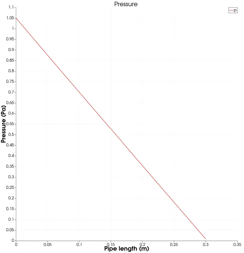
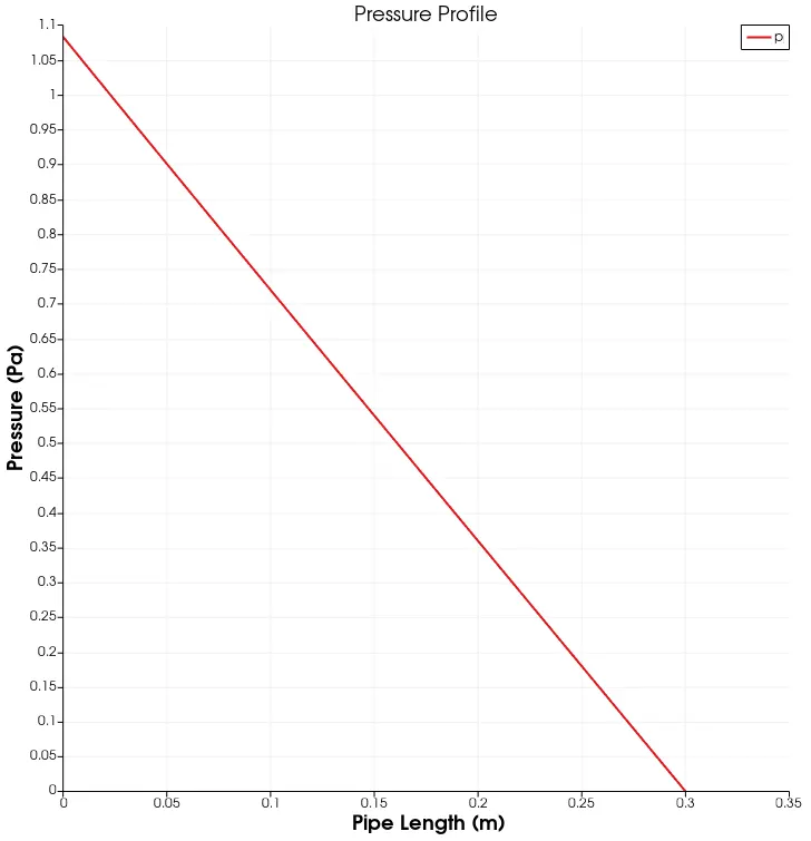
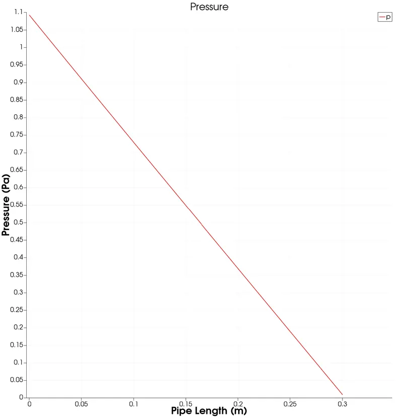
Pressure Profile:-
Wedge Symmetry
`10^o`:
`25^o`:
`45^o`:
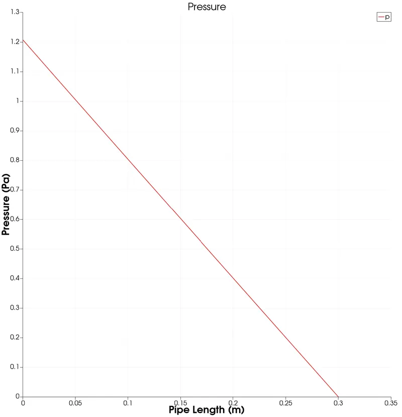
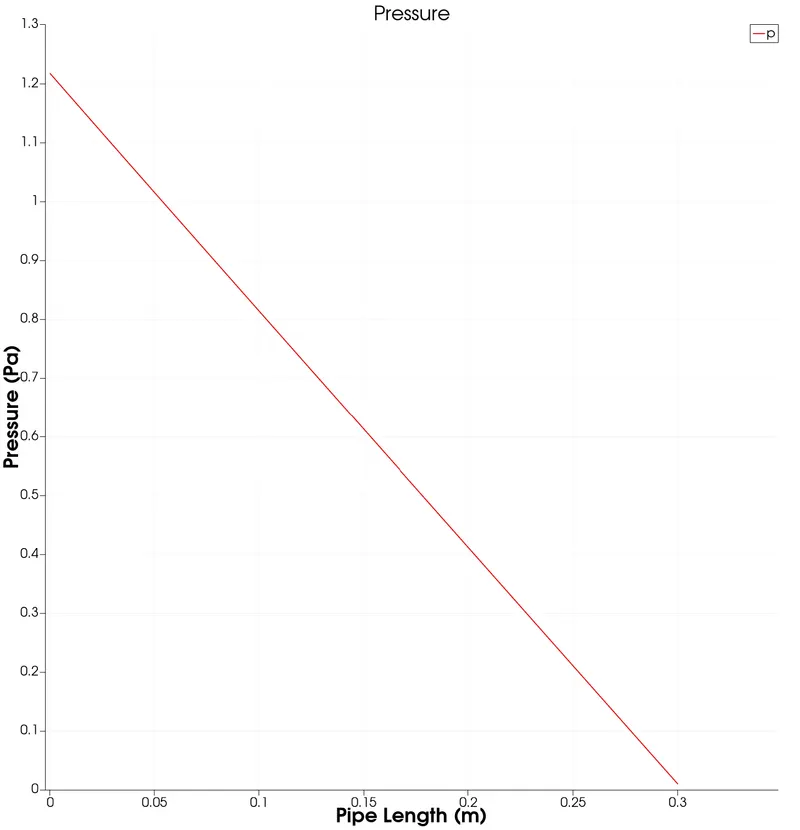
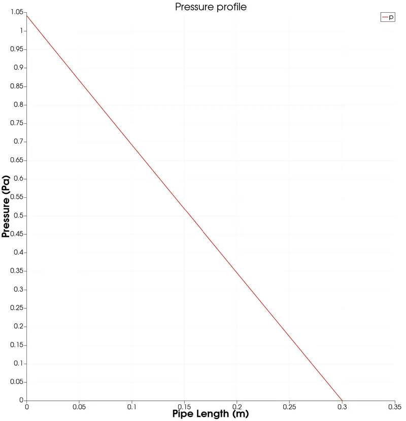
Now we observe the pressure profiles captured along the pipe for different angles and boundary conditions. And it is clearly evident that the pressure is decreasing as we move along the domain. This tells us that the pressure is high at the pipe entrance due to the non-uniformity in the velocity gradient due to high shear stress as we have observed in the above velocity profiles. The pressure naturally decreases as the velocity moves towards more uniformity where the boundary layers are uniform in nature. As the flow moves on to the fully developed flow region, we see constant and uniform decrease in the pressure gradient compensating for the viscous forces in the flow. So, we can concur that the pressure drop is due to the viscous forces of the fluid.
Note:
It is important to understand that the pressure drop has to be captured in the fully developed flow region. It dosen't make any sense if we capture the profile over the entire pipe length. Although the trend would be the same, the profiles are still developing in the hydrodynamic entry region. So in order to extract the accurate pressure drop, we need to concentrate only on the fully developed flow region.
Shear Stress Profile:-
Wedge Symmetry
`10^o`:
`25^o`:
`45^o`:
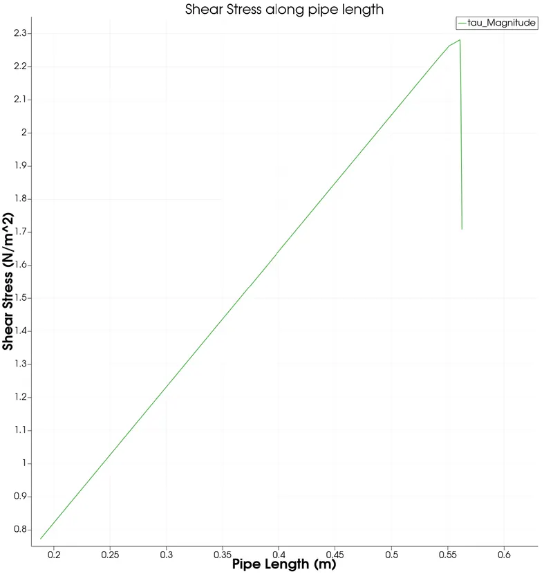
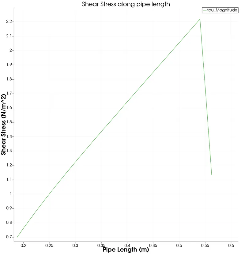
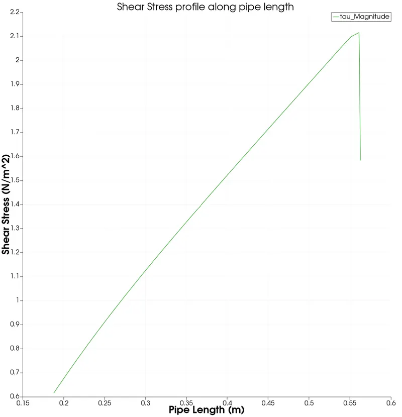
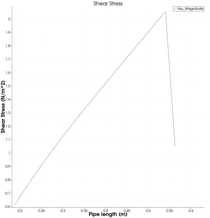
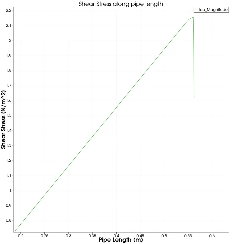
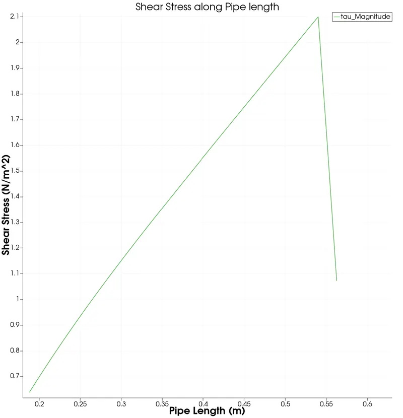
The above Shear Stress plots were taken falong the entire pipe length. For all the cases, the shear stress is very low at the axis and peaks in the fully developed region near the walls. This phenomenon of high shear stress is due to the no-slip condition which happens due to high viscous forces at the pipe wall.
Validation Studies:
Now, we will extract the numerical solution data from Paraview and process them in Matlab and compare them with the analytical data. This is done so that we can understand how accurate our numerical solutions are when compared with the analytical solution. The only change in the code would be the different case files for the particular case(Wedge and Symmetry BC). Here, we are comparing the cases on the basis of the angles taken for the Wedge and the Symmetry boundary conditions. The Matlab code is given below
Post-process Matlab code:
clear all
close all
clc

% Input Data (meters)
D = 0.0025; % Diameter
R = D/2; % Radius
Re = 2100; % Reynolds Number
L_e = 0.05*Re*D; % Hydrodynamic Entry length
L = 0.3 + L_e; % Total Length
L_fd = L - L_e % Fully Developed Flow Region Length
theta = 3; % Wedge Angle
mu = 0.000890; % (Pa.s) Dynamic Viscosity
rho = 997; % (kg/m^3) Density of Water
nu = mu/rho; % (m^2/s) Kinematic viscosity

% Reading and Extracting Velocity Data from Paraview
% Wedge Boundary Condition Data
f1 = fopen('w10-velocity.csv','r');
A = fgetl(f1);
for i = 1:1000
    B = fgetl(f1);
    C = strsplit(B,',');
    Vel_n_w(i) = C(2);
    Len_n_w(i) = C(1);
end
Vel_n_w = str2double(Vel_n_w');
Len_n_w = str2double(Len_n_w');

%Reading and Extracting Pressure Data from Paraview
f2 = fopen('w10-pressure.csv','r');
A = fgetl(f2);
for i = 1:1000
    B = fgetl(f2);
    C = strsplit(B,',');
    Press_n_w(i) = C(2);
    Len_n2_w(i) = C(1);
end
Press_n_w = str2double(Press_n_w');
Len_n2_w = str2double(Len_n2_w');

%Reading and Extracting Shear Stress Data from Paraview
f3 = fopen('w10-tau.csv','r');
A = fgetl(f3);
for i = 1:1000
    B = fgetl(f3);
    C = strsplit(B,',');
    tau_n_w(i) = C(2);
    Len_n3_w(i) = C(1);
end
tau_n_w = str2double(tau_n_w');
Len_n3_w = str2double(Len_n3_w');

% Symmetry Boundary Condition Data
f4 = fopen('s10-velocity.csv','r');
A = fgetl(f4);
for i = 1:1000
    B = fgetl(f4);
    C = strsplit(B,',');
    Vel_n_s(i) = C(2);
    Len_n_s(i) = C(1);
end
Vel_n_s = str2double(Vel_n_s');
Len_n_s = str2double(Len_n_s');

%Reading and Extracting Pressure Data from Paraview
f5 = fopen('s10-Pressure.csv','r');
A = fgetl(f5);
for i = 1:1000
    B = fgetl(f5);
    C = strsplit(B,',');
    Press_n_s(i) = C(2);
    Len_n2_s(i) = C(1);
end
Press_n_s = str2double(Press_n_s');
Len_n2_s = str2double(Len_n2_s');

%Reading and Extracting Shear Stress Data from Paraview
f6 = fopen('s10-tau.csv','r');
A = fgetl(f6);
for i = 1:1000
    B = fgetl(f6);
    C = strsplit(B,',');
    tau_n_s(i) = C(2);
    Len_n3_s(i) = C(1);
end
tau_n_s = str2double(tau_n_s');
Len_n3_s = str2double(Len_n3_s');

r = linspace(0,R,1000); % Radial Distance
% Hagen poiseuille's Solution
V_avg = (Re*mu)/(rho*D); % Average velocity
u_max = 2*V_avg; % Maximum Velocity
V_r = u_max*(1-(r.^2./R^2));


% Hagen-Poiseuille Equations for Pressure Drop
P_len = linspace(0,L_fd,1000); % Pipe Length
for i = 1:length(P_len)
    delta_p(i) = (8*mu*P_len(i)*V_avg)/R^2; % Pressure Drop
    k_press(i) = delta_p(i)/rho; % Kinematic Pressure
end

k_press = fliplr(k_press);

% Analytical Shear Stress calculation
for i=1:length(r)
   tau_an(i)=(2*mu*u_max*r(i))/R^2;
end


figure(1)
plot(r,V_r,'r','linewidth',1) % Anaytical Data
hold on
plot(Len_n_w,Vel_n_w,'--','color','b','linewidth',1) % Numerical Data for Wedge BC
hold on
plot(Len_n_s,Vel_n_s,'--','color','k','linewidth',1) % Numerical Data for Symmetry BC
title('Velocity: Numerical vs Analytical Data')
xlabel('Radial Length (m)')
ylabel('Velocity in m/s')
legend('Analytical Method','Numerical Method for Wedge BC','Numerical Method for Symmetry BC')
grid on

figure(2)
plot(P_len,k_press,'r','linewidth',1) % Analytical Data
hold on
plot(Len_n2_w,Press_n_w,'--','color','b','linewidth',1) % Numerical Data for Wedge BC
hold on
plot(Len_n2_s,Press_n_s,'--','color','k','linewidth',1) % Numerical Data for Symmetry BC
title('Pressure: Numerical vs Analytical Data')
xlabel('Radial Length (m)')
ylabel('Pressure (Pa)')
legend('Analytical Method','Numerical Method for Wedge BC','Numerical Method for Symmetry BC')
grid on

figure(3)
plot(r,tau_an,'r','linewidth',1) % Analytical Data
hold on
plot(Len_n3_w,tau_n_w,'--','color','b','linewidth',1) % Numerical Data for Wedge BC
hold on
plot(Len_n3_s,tau_n_s,'--','color','k','linewidth',1) % Numerical Data for Symmetry BC
title('Shear Stress: Numerical vs Analytical Data')
xlabel('Radial Length (m)')
ylabel('Shear Stress (N/m^2)')
legend('Analytical Method','Numerical Method for Wedge BC','Numerical Method for Symmetry BC')
grid on
In the above code, we are reading the extracted data files from paraview and parse them to plot with the analytical solution. For different cases, we just change the name of the data file.
The formulae used in the analytical solution are given below
Average Velocity:
`V_(avg)=(Re*mu)/(rho*D)`
Radius at various radial lengths at the fully developed region:
`V_r = 2*V_(avg)*(1-(r^2)/R^2)`
Pressure drop across the pipe length:
`Deltap = (8*mu*V_(avg)*L)/R^2`
Kinematic Pressure:
`K_(press) = (DeltaP)/rho`
Shear Stress:
`tau = (2*mu*u_(max)*r)/R`
All of the following plots show the comparison of Numerical to Analytical studies for Velocity, Pressure and Shear stress respectively
For `10^o` degrees:
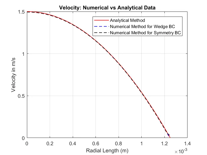
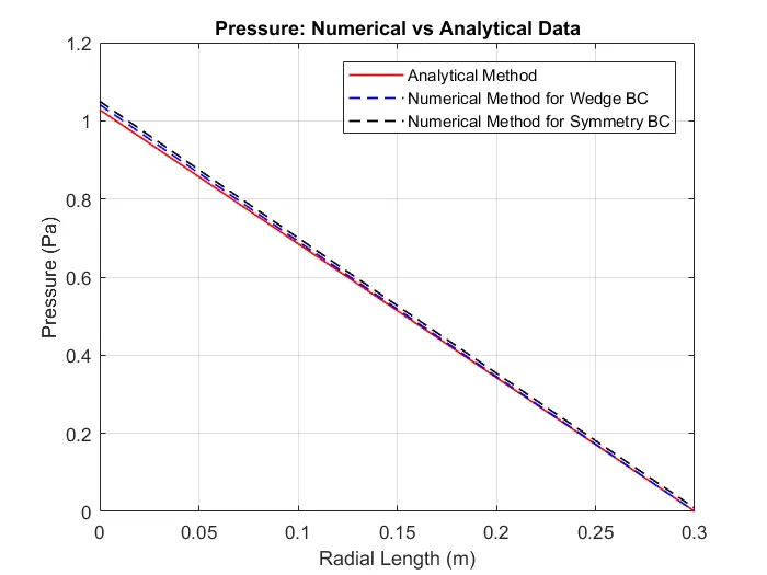
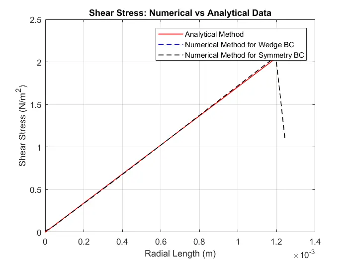
In the above plots, we can see that the numerical and the the analytical solutions are similar. When compared with the actual values, we will see that an error will exist but would be negligible which is of
`0.01%`.
For `25^o` degrees:
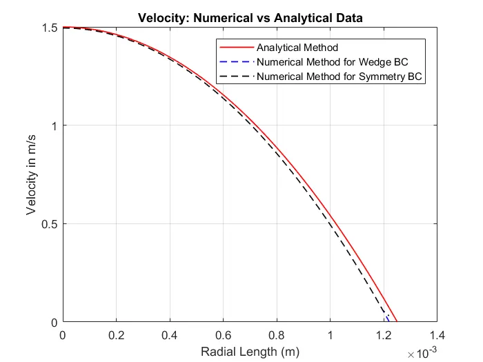
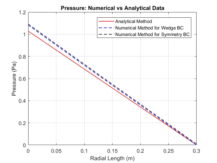
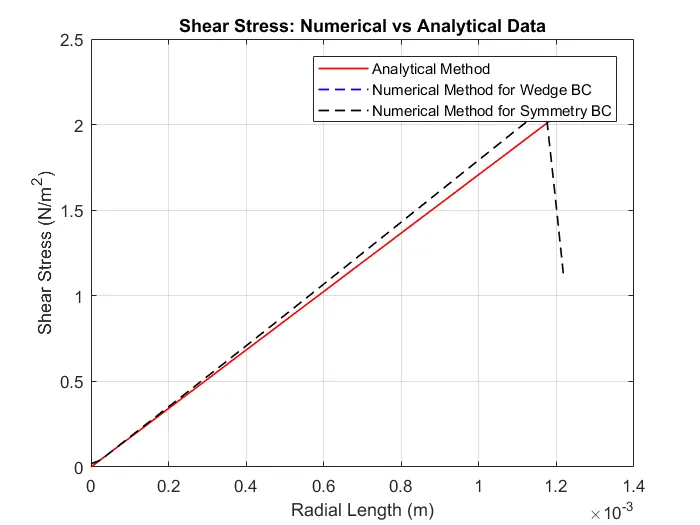
In the above plots, we can see that the trends are almost close to each other with visible errors. This deviation is due to the increment of the angle i.e we are using the same mesh and the simulation time (refer ControlDict) as taken for the `10^o` case. If we go into detail, it is due to the bigger angle for the wedge and the symmetry boundary conditions, same mesh methodology and simulation time, we find the error in the above comparison plots. Therefore, if the mesh were more finer or the time step smaller respectively, we would get very close trends for the above parameters of Velocity, Pressure and Shear Stress.
For `45^o` degrees:
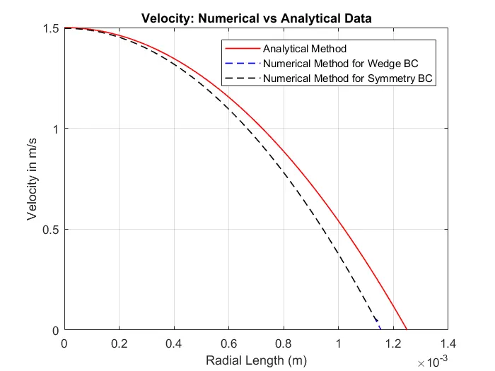
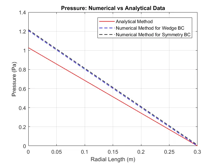
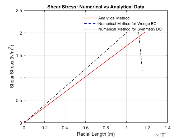
In the above plots, we can see that the trends are close to each other with visible errors. This deviation is due to the increment of the angle i.e we are using the same mesh and the simulation time (refer ControlDict) as taken for the `10^o` or the `25^o` case. If we go into detail, it is due to the bigger angle for the wedge and the symmetry boundary conditions, same mesh methodology and simulation time, we find the error in the above comparison plots. Therefore, if the mesh were more finer or the time step smaller respectively, we would get very close trends for the above parameters of Velocity, Pressure and Shear Stress.
Conclusion:-
We have automated the process of creating the blockMeshdict file for our simulations using Matlab.
We have seen that the data obtained from the numerical simulation is close to the analytical solutions.
References:-
Fluid Mechanics Fundamentals and Applications by Yunus Cengel, John Cimbala
https://en.wikipedia.org/wiki/Hagen%E2%80%93Poiseuille_equation