Week 12 - Validation studies of Symmetry BC vs Wedge BC in OpenFOAM vs Analytical H.P equation
- Aim: To study the effect of the wedge angle and the Boundary Conditions on the simulation of an axisymmetric laminar flow in a cylindrical pipe.
- Theoretical Introduction:
Axi-symmetric flow: A flow pattern is axisymmetric when it is identical in every plane that passes through a certain straight-line. The straight-line in question is referred to as the symmetry axis.
Every longitudinal plane through the axis would exhibit the same streamline pattern.
Laminar Flow: In fluid dynamics, laminar flow is characterized by fluid particles following smooth paths in layers, with each layer moving smoothly past the adjacent layers with little or no mixing. At low velocities, the fluid tends to flow without lateral mixing, and adjacent layers slide past one another like playing cards. There are no cross-currents perpendicular to the direction of flow, nor eddies or swirls of fluids. In laminar flow, the fluid particles' motion is very orderly, with particles close to a solid surface moving in straight lines parallel to that surface.
Laminar flow is a flow regime characterized by high momentum diffusion and low momentum convection.
When a fluid flows through a closed channel such as a pipe or between two flat plates, either of two types of flow may occur depending on the fluid's velocity and viscosity: laminar flow or turbulent flow. Laminar flow occurs at lower velocities, below a threshold at which the flow becomes turbulent. The velocity is determined by a dimensionless parameter characterizing the flow called the Reynolds number, which also depends on the viscosity and density of the fluid and dimensions of the channel.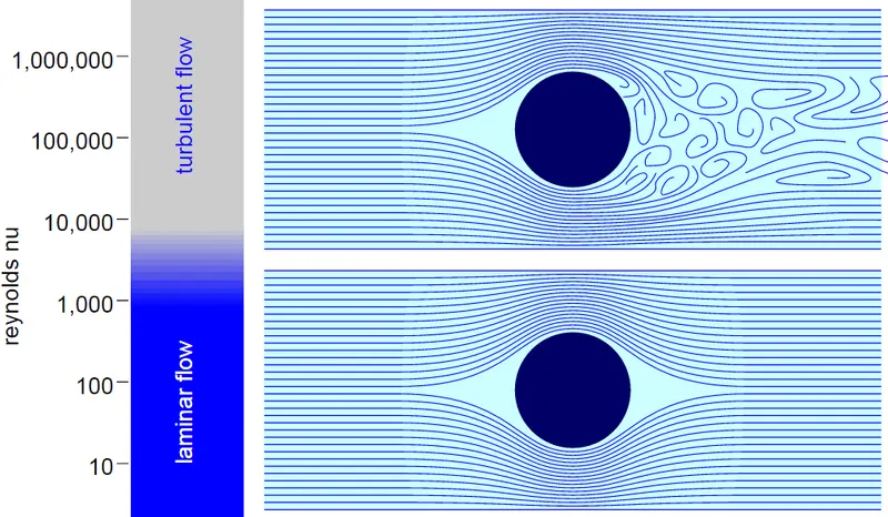
Comparison between Turbulent and Laminar Flow.
Reynolds Number: The Reynolds number (Re) helps predict flow patterns in different fluid flow situations. At low Reynolds numbers, flows tend to be dominated by laminar (sheet-like) flow, while at high Reynolds numbers, flows tend to be turbulent. The turbulence results from differences in the fluid's speed and direction, which may sometimes intersect or even move counter to the flow's overall direction (eddy currents). These eddy currents begin to churn the flow, using up energy in the process, which for liquids increases the chances of cavitation. Reynolds numbers are an important dimensionless quantity in fluid mechanics.
The Reynolds number has wide applications, ranging from liquid flow in a pipe to the passage of air over an aircraft wing. It is used to predict the transition from laminar to turbulent flow and is used in the scaling of similar but different-sized flow situations, such as between an aircraft model in a wind tunnel and the full-size version. The predictions of the onset of turbulence and the ability to calculate scaling effects can be used to help predict fluid behaviour on a larger scale, such as in local or global air or water movement and thereby the associated meteorological and climatological effects. - Procedure:
1. The procedure for this challenge involves editing the previously made MATLAB code and changing the input and the Boundary Conditions in OpenFoam.
2. In the Automated BlockMeshDict file, we need to edit the wedge angle for one particular boundary condition. The angles at which we are performing the simulation and then later studying the simulation results are:
a. 10o">10o10
b. 25o">25o25
c. 45o">45o45
45o">Matlab Code :-
clear all
close all
clc

%Inputs:
l= 1.5;         %Length of the pipe.
theta = 45.0;    %Wedge angle.
d = 0.01;       %Diameter of the pipe.
c = 1.0;        %Conversion Factor.
r = d/2;        %Radius of the Cylinder.
nx = 500;       %number of Mesh points in x-direction on the block.
ny= 25;         %Number of Mesh points in the y-direction on the block.
nz= 1;          %number of Mesh Points in the z-direction on the block.
gx = 1;         %Grading along the x-direction.
gy = 1;         %Grading along the y-direction.
gz = 1;         %Grading along the z-direction.


f1 = fopen('BlockMeshDict.txt','w');
fprintf(f1,'/*--------------------------------*- C++ -*----------------------------------*n');
fprintf(f1,'  =========                 | n');
fprintf(f1,'        /  F ield         | OpenFOAM: The Open Source CFD Toolbox n');
fprintf(f1,'       /   O peration     | Website:  https://openfoam.org n');
fprintf(f1,'      /    A nd           | Version:  8 n');
fprintf(f1,'     /     M anipulation  | n');
fprintf(f1,'/*------------------------------------------------------------------*/ n');
fprintf(f1, 'FoamFile n');
fprintf(f1,'{ n');
fprintf(f1,'    version     2.0; n');
fprintf(f1,'    format      ascii; n' );
fprintf(f1,'    class       dictionary; n');
fprintf(f1,'    object      blockMeshDict; n');
fprintf(f1,'} n');
fprintf(f1,'// * * * * * * * * * * * * * * * * * * * * * * * * * * * * * * * * * * * * * // n');

fprintf(f1,'convertToMeters %0.1f; n',c);
fprintf(f1,'n');
fprintf(f1,'vertices n');
fprintf(f1,'( n');
fprintf(f1,'(0 0 0) n');
fprintf(f1,'(%0.6f %0.6f %0.3f)n',r*sind(theta/2),r*cosd(theta/2),0);
fprintf(f1, '(%0.6f %0.6f %0.3f)n',-r*sind(theta/2),r*cosd(theta/2),0);
fprintf(f1,'(0 0 %0.3f) n',-l);
fprintf(f1,'(%0.6f %0.6f %0.3f)n',r*sind(theta/2),r*cosd(theta/2),-l);
fprintf(f1, '(%0.6f %0.6f %0.3f)n',-r*sind(theta/2),r*cosd(theta/2),-l);
fprintf(f1,'); n');
fprintf(f1,'n');

fprintf(f1,'blocks n');
fprintf(f1,'( n');
fprintf(f1,'hex (0 3 5 2 0 3 4 1) (%0.0f %0.0f %0.0f) simpleGrading (%0.0f %0.0f %0.0f) n',nx,ny,nz,gx,gy,gz);
fprintf(f1,'); n');
fprintf(f1,'n');

fprintf(f1,'edges n');
fprintf(f1,'( n');
fprintf(f1,'); n');
fprintf(f1,'n');

fprintf(f1,'boundary n');
fprintf(f1,'( n');
fprintf(f1,'in n');
fprintf(f1,'{ n');
fprintf(f1,'type patch; n');
fprintf(f1,'faces n');
fprintf(f1,'( n');
fprintf(f1,'(0 1 2 0) n');
fprintf(f1,'); n');
fprintf(f1,'} n');

fprintf(f1,'out n');
fprintf(f1,'{ n');
fprintf(f1,'type patch; n');
fprintf(f1,'faces n');
fprintf(f1,'( n');
fprintf(f1,'(3 5 4 3) n');
fprintf(f1,'); n');
fprintf(f1,'} n');

fprintf(f1,'ft n');
fprintf(f1,'{ n');
fprintf(f1,'type wedge; n');
fprintf(f1,'faces n');
fprintf(f1,'( n');
fprintf(f1,'(0 3 4 1) n');
fprintf(f1,'); n');
fprintf(f1,'} n');

fprintf(f1,'bk n');
fprintf(f1,'{ n');
fprintf(f1,'type wedge; n');
fprintf(f1,'faces n');
fprintf(f1,'( n');
fprintf(f1,'(3 0 2 5) n');
fprintf(f1,'); n');
fprintf(f1,'} n');

fprintf(f1,'top n');
fprintf(f1,'{ n');
fprintf(f1,'type wall; n');
fprintf(f1,'faces n');
fprintf(f1,'( n');
fprintf(f1,'(5 2 1 4) n');
fprintf(f1,'); n');
fprintf(f1,'} n');

fprintf(f1,'axis n');
fprintf(f1,'{ n');
fprintf(f1,'type empty; n');
fprintf(f1,'faces n');
fprintf(f1,'( n');
fprintf(f1,'(0 3 3 0) n');
fprintf(f1,'); n');
fprintf(f1, '} n');

fprintf(f1,'); n');
fprintf(f1,'n');

fprintf(f1,'mergePatchPairs n');
fprintf(f1,'( n');
fprintf(f1,'); n');
fprintf(f1,'n');
fprintf(f1,'// ************************************************************************* // n');


%END
The code for Symmetry Boundary Condition at a wedge angle of 45 deg is as follows:
clear all
close all
clc
%Inputs:
l= 1.5; %Length of the pipe.
theta = 45.0; %Wedge angle.
d = 0.01; %Diameter of the pipe.
c = 1.0; %Conversion Factor.
r = d/2; %Radius of the Cylinder.
nx = 500; %number of Mesh points in x-direction on the block.
ny= 25; %Number of Mesh points in the y-direction on the block.
nz= 3; %number of Mesh Points in the z-direction on the block.
gx = 1; %Grading along the x-direction.
gy = 1; %Grading along the y-direction.
gz = 1; %Grading along the z-direction.
f1 = fopen('BlockMeshDict.txt','w');
fprintf(f1,'/*--------------------------------*- C++ -*----------------------------------*n');
fprintf(f1,' ========= | n');
fprintf(f1,' / F ield | OpenFOAM: The Open Source CFD Toolbox n');
fprintf(f1,' / O peration | Website: https://openfoam.org n');
fprintf(f1,' / A nd | Version: 8 n');
fprintf(f1,' / M anipulation | n');
fprintf(f1,'/*------------------------------------------------------------------*/ n');
fprintf(f1, 'FoamFile n');
fprintf(f1,'{ n');
fprintf(f1,' version 2.0; n');
fprintf(f1,' format ascii; n' );
fprintf(f1,' class dictionary; n');
fprintf(f1,' object blockMeshDict; n');
fprintf(f1,'} n');
fprintf(f1,'// * * * * * * * * * * * * * * * * * * * * * * * * * * * * * * * * * * * * * // n');
fprintf(f1,'convertToMeters %0.1f; n',c);
fprintf(f1,'n');
fprintf(f1,'vertices n');
fprintf(f1,'( n');
fprintf(f1,'(0 0 0) n');
fprintf(f1,'(%0.6f %0.6f %0.3f)n',r*sind(theta/2),r*cosd(theta/2),0);
fprintf(f1, '(%0.6f %0.6f %0.3f)n',-r*sind(theta/2),r*cosd(theta/2),0);
fprintf(f1,'(0 0 %0.3f) n',-l);
fprintf(f1,'(%0.6f %0.6f %0.3f)n',r*sind(theta/2),r*cosd(theta/2),-l);
fprintf(f1, '(%0.6f %0.6f %0.3f)n',-r*sind(theta/2),r*cosd(theta/2),-l);
fprintf(f1,'); n');
fprintf(f1,'n');
fprintf(f1,'blocks n');
fprintf(f1,'( n');
fprintf(f1,'hex (0 3 5 2 0 3 4 1) (%0.0f %0.0f %0.0f) simpleGrading (%0.0f %0.0f %0.0f) n',nx,ny,nz,gx,gy,gz);
fprintf(f1,'); n');
fprintf(f1,'n');
fprintf(f1,'edges n');
fprintf(f1,'( n');
fprintf(f1,'); n');
fprintf(f1,'n');
fprintf(f1,'boundary n');
fprintf(f1,'( n');
fprintf(f1,'in n');
fprintf(f1,'{ n');
fprintf(f1,'type patch; n');
fprintf(f1,'faces n');
fprintf(f1,'( n');
fprintf(f1,'(0 1 2 0) n');
fprintf(f1,'); n');
fprintf(f1,'} n');
fprintf(f1,'out n');
fprintf(f1,'{ n');
fprintf(f1,'type patch; n');
fprintf(f1,'faces n');
fprintf(f1,'( n');
fprintf(f1,'(3 5 4 3) n');
fprintf(f1,'); n');
fprintf(f1,'} n');
fprintf(f1,'ft n');
fprintf(f1,'{ n');
fprintf(f1,'type symmetry; n');
fprintf(f1,'faces n');
fprintf(f1,'( n');
fprintf(f1,'(0 3 4 1) n');
fprintf(f1,'); n');
fprintf(f1,'} n');
fprintf(f1,'bk n');
fprintf(f1,'{ n');
fprintf(f1,'type symmetry; n');
fprintf(f1,'faces n');
fprintf(f1,'( n');
fprintf(f1,'(3 0 2 5) n');
fprintf(f1,'); n');
fprintf(f1,'} n');
fprintf(f1,'top n');
fprintf(f1,'{ n');
fprintf(f1,'type wall; n');
fprintf(f1,'faces n');
fprintf(f1,'( n');
fprintf(f1,'(5 2 1 4) n');
fprintf(f1,'); n');
fprintf(f1,'} n');
fprintf(f1,'axis n');
fprintf(f1,'{ n');
fprintf(f1,'type empty; n');
fprintf(f1,'faces n');
fprintf(f1,'( n');
fprintf(f1,'(0 3 3 0) n');
fprintf(f1,'); n');
fprintf(f1, '} n');
fprintf(f1,'); n');
fprintf(f1,'n');
fprintf(f1,'mergePatchPairs n');
fprintf(f1,'( n');
fprintf(f1,'); n');
fprintf(f1,'n');
fprintf(f1,'// ************************************************************************* // n');
%END So, we must run the simulation and plot the necessary graphs at all the Boundary Conditions' angles, i.e. Wedge Boundary conditions and the Symmetry Boundary Condition. We must make use of the plot over line command to study how the shear force is varying with a change in the distance along the radial direction. In contrast, the Pressure drop is to be studied in the fully developed region along the Axial Direction.
To plot the line, we must use the plot over line command. This will help us study the data variation along that line.
The line is drawn, as shown below:
Result:
1. The first simulation comparison is with the Wedge Boundary condition. Within this Boundary Condition, the simulation comparison for all the above-mentioned angles is as follows.
We will compare the Shear Stress developed for both the boundary conditions at all three angles.
a.Shear Stress Variation with respect to the Radial Distance.
The Shear Stress plot for both the Boundary Conditions, the wedge Boundary Condition and the Symmetry Boundary Condition are shown at 10degrees. We can see that when we apply the Symmetry Boundary Condition, the slope of the curve is much higher than when we apply the Wedge Boundary Condition. So, when we apply the Symmetry Boundary Condition, the Mesh becomes 3D, and the computation is done for all three global axes. This affects the calculation as well. The peak value in the Wedge Boundary Condition is approximately 0.145 units, but whereas when we apply the Symmetry Boundary Condition, the peak value touches around 0.140units.
The graph shown above is comparing the Shear Stress for both the boundary conditions for when the wedge angle is 25degrees.
Similarly, we plot and study all the graphs, as shown below:
b. Velocity Variation with respect to Radial Distance.
Velocity variation at 10degrees for the two Boundary Conditions.
Velocity variation at 25 degrees for the two Boundary Conditions.
Velocity variation at 45 degrees for the two Boundary Conditions.
c. Pressure Drop across the axial Distance
Pressure drop at 10 degrees across the Axial Distance.
Pressure drop at 25 degrees across the Axial Distance.
Pressure drop at 45 degrees across the Axial Distance.
Validation:
a.Validation of Maximum Pressure drop in the Fully developed Region.
These graphs depict the change in the various parameters for both the Boundary Conditions, and we can compare these quantities properly.
Like for example, we can compare the pressure drop from the graph and the pressure drop that we get analytically.
From the graph, we can see that the maximum value - minimum value = 0.26 - 0.13 = 0.13units = 130Pascal.
And, when we calculate it analytically, we know that the formula is :
△P=Vavg⋅μ⋅LD2△
We know all the values, they are as follows:
vavg=0.21units
μ=0.01924
L=0.2units
D=0.1units
For a Kinematic Viscosity of 1.924e-5(Used in the simulation), the Dynamic Viscosity is 1.924e-5*1000 = 1.924e-2units.
Calculating using these values, we get: △P= 0.129units
The error between the Analytical value and the value obtained from the graph is (0.13-0.129) / (0.129) = 0.7%, which is under the tolerance limit of 5%.
Now, because the error is under tolerance, we can conclude that the simulation has reached a Steady State.
b.Validation of the Maximum Velocity
Now, if we wish to compare the Maximum velocity from the graph, we can see that the value is 0.42units.
According to the Analytical formula, we know that the maximum velocity must be: 2⋅vavg
And our Vavg is 0.21units; hence the analytical value will be 0.42units that matches the value that we get from the graph.
c. To validate the Hydrodynamic length with the Numerical Result.
So, In fluid dynamics, the entrance length is the distance a flow travels after entering a pipe before the flow becomes fully developed. Entrance length refers to the length of the entry region, the area following the pipe entrance where effects originating from the interior wall of the pipe propagate into the flow as an expanding boundary layer.
Velocity profile before the Hydrodynamic Length
Velocity after the Hydrodynamic length
d. Shear Stress Plot:
Shear Stress is the maximum near the wall because of the friction that the wall has. But, as we move away from the wall, the Shear Force decreases, and it can be confirmed with the graph above.
According to the Analytically calculated profile, the graph is:
u(r)=2⋅vavg⋅(1−r2R2)
And we know that this profile also gives out a Parabolic curve similar to the one we have gotten in the graph.
e. Comparison between the two Boundary Conditions.
We have performed Simulation for two Boundary Conditions; those are Symmetry Boundary Condition and the Wedge Boundary Condition.
During the Wedge Boundary condition simulation, the simulation across the arc of the wedge is not done, but whereas in the case of Symmetry Boundary Condition, the calculation across the arc of the wedge is done; hence the simulation time is higher in that case. The Courant number is increasing slightly in the case of wedge Boundary Condition and hence the Symmetry Boundary Condition will be slightly more accurate. The Symmetry Boundary condition considers the Mesh as 3D and the calculation is done along all the three global axes.
We understand the results should not change due to the change in the Boundary conditions, and this is because the Physics of the problem does not change and remains the same.
Conclusion:
In conclusion, I would like to state that this challenge helped me understand the difference between the two boundary conditions and how to simulate them as per the need of the problem that we will be simulating.