Symmetry vs Wedge vs HP equation

problem specification:

let us assume a cylindrical pipe of 0.01m diameter and length 2m

Fluid flowing with a velocity of 15m/sec with a kinematic viscosity of 1e-4 sqm/sec .

d = 0.01m.

nu = 1e-4 sqm/sec.

v = 15m/sec.

l = 2m.

rho = 1000 kg/cubicm.

mu = 10 Ns/sqm.

outlet is open to atmospheric pressure.

The Renolds number will be 1500

Hagen poiseuille's flow

In nonideal fluid dynamics the Hagen–Poiseuille equation, also known as the Hagen–Poiseuille law, Poiseuille law or Poiseuille equation, is a physical law that gives the pressure drop in an incompressible and Newtonian fluid in laminar flow flowing through a long cylindrical pipe of constant cross-section. It can be successfully applied to airflow in lung alveoli, or the flow through a drinking straw or a hypodermic needle.

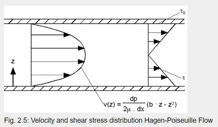
The equation assumes that the fluid is incompressible and Newtonian; the flow is laminar through a pipe of the constant circular cross-section that is substantially longer than its diameter, and there is no acceleration of fluid in the pipe. For velocities and pipe diameters above a threshold, actual fluid flow is not laminar but turbulent, leading to larger pressure drops than calculated by the Hagen–Poiseuille equation.

The specific calculation of the Reynolds number, and the values where laminar flow occurs, will depend on the geometry of the flow system and flow pattern. The common example flows through a pipe, where the Reynolds number is defined as

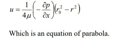
velocity distribution in the radial direction for fully developed laminar flow in a pipe of constant diameter:

shear stress distribution in the radial direction for fully developed laminar flow in a pipe of constant diameter:

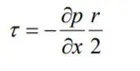
which is linear, zero at a centre and maximum at walls as shown in the figure above.

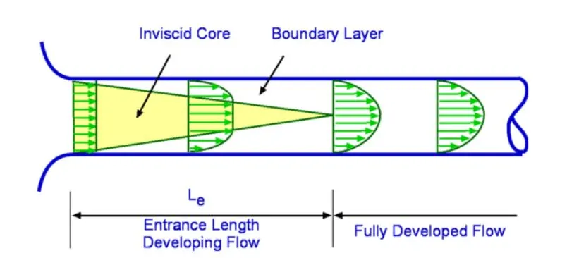
The fully developed flow starts after the entrance length which can be calculated using the equation.

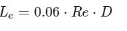
To get correct velocity and shear stress profiles we should measure the profiles after this entrance length.

Matlab code to generate blockmesh file.

clear all
close all
clc

%% MATLAB program for auto-generation of blockmesh file in OpenFoam %%

d = 0.01; % diameter

L_t = 2; %total length
r = d/2; % radius
theta = 45; %degree(input according to the need)

%% Calculating the vertices of the wedge
v0 = [ 0 0 0 ];
v1 = [ L_t 0 0 ];
v2 = [ 0 -r*sind(theta) r*cosd(theta)];
v3 = [ L_t -r*sind(theta) r*cosd(theta)];
v4 = [ L_t r*sind(theta) r*cosd(theta)];
v5 = [ 0 r*sind(theta) r*cosd(theta)];


%% String format specifying for Blockmesh file %%
head1 = '/*--------------------------------*- C++ -*----------------------------------*';
head2 = '| =========                 |                                                 |';
head3 = '|       /  F ield         | OpenFOAM: The Open Source CFD Toolbox           |';
head4 = '|      /   O peration     | Version:  7                                     |';
head5 = '|     /    A nd           | Website:  https://openfoam.org                  |';
head6 = '|    /     M anipulation  |                                                 |';
head7 = '*---------------------------------------------------------------------------*/';


b4 = blanks(4);
b8 = blanks(8);
b12 = blanks(12);
b16 = blanks(16);

dict1 = '    version     2.0;';
dict2 = '    format      ascii;';
dict3 = '    class       dictionary;';
dict4 = '    object      blockMeshDict;';
dict5 = '// * * * * * * * * * * * * * * * * * * * * * * * * * * * * * * * * * * * * * //';

conv = 'convertToMeters 1;';

vertex1 = 'vertices';

blocks1 = 'hex (0 1 1 0 2 3 4 5) (200 3 50) simpleGrading (1 1 0.2)';

footer = '// ************************************************************************* //';

%% Creting blockMesh dict for OepnFOAM %%

f1 = fopen('blockMeshdict.txt','w')

% Printing the headder %%

fprintf(f1,'%sn' ,head1);
fprintf(f1,'%sn' ,head2);
fprintf(f1,'%sn' ,head3);
fprintf(f1,'%sn' ,head4);
fprintf(f1,'%sn' ,head5);
fprintf(f1,'%sn' ,head6);
fprintf(f1,'%sn' ,head7);

fprintf(f1,'FoamFilen{n' );

fprintf(f1,'%s%sn', b4,dict1);
fprintf(f1,'%s%sn', b4,dict2);
fprintf(f1,'%s%sn', b4,dict3);
fprintf(f1,'%s%sn', b4,dict4);
fprintf(f1,'}n%s%snnn', b4,dict5);

fprintf(f1,'%sn', conv);

%% Printing the vertices %%

fprintf(f1,'verticesn(n');
fprintf(f1,'%s(%d %d %d)n', b4,v0(1),v0(2),v0(3));
fprintf(f1,'%s(%d %d %d)n', b4,v1(1),v1(2),v1(3));
fprintf(f1,'%s(%d %f %f)n', b4,v2(1),v2(2),v2(3));
fprintf(f1,'%s(%d %f %f)n', b4,v3(1),v3(2),v3(3));
fprintf(f1,'%s(%d %f %f)n', b4,v4(1),v4(2),v4(3));
fprintf(f1,'%s(%d %f %f)n', b4,v5(1),v5(2),v5(3));
fprintf(f1,');n');

%% Printing the blocks %%

fprintf(f1,'nblocksn(n');
fprintf(f1,'%s%sn', b4,blocks1);
fprintf(f1,');n');

%% Printing edges %%

fprintf(f1,'nedgesn(n');
fprintf(f1,'%sarc 2 5 (0 0 %0.3f)n', b4,r);
fprintf(f1,'%sarc 3 4 (%0.2f 0 %0.3f)n', b4,L_t,r);
fprintf(f1,');n');

%% Printing boundary %%

fprintf(f1,'nboundaryn(n');


fprintf(f1,'%sinletn%s{n', b4,b4);
fprintf(f1,'%stype patch;n', b8);
fprintf(f1,'%sfacesn%s(n', b8,b8);
fprintf(f1,'%s(0 2 5 0)n%s);n%s}n', b12,b8,b4);


fprintf(f1,'%saxisn%s{n', b4,b4);
fprintf(f1,'%stype empty;n', b8);
fprintf(f1,'%sfacesn%s(n', b8,b8);
fprintf(f1,'%s(0 1 1 0)n%s);n%s}n', b12,b8,b4);

fprintf(f1,'%swalln%s{n', b4,b4);
fprintf(f1,'%stype wall;n', b8);
fprintf(f1,'%sfacesn%s(n', b8,b8);
fprintf(f1,'%s(2 3 4 5)n%s);n%s}n', b12,b8,b4);

fprintf(f1,'%soutletn%s{n', b4,b4);
fprintf(f1,'%stype patch;n', b8);
fprintf(f1,'%sfacesn%s(n', b8,b8);
fprintf(f1,'%s(1 3 4 1)n%s);n%s}n', b12,b8,b4);

fprintf(f1,'%saxi_symm-fn%s{n', b4,b4);
fprintf(f1,'%stype symmetry;n', b8);
fprintf(f1,'%sfacesn%s(n', b8,b8);
fprintf(f1,'%s(0 1 4 5)n%s);n%s}n', b12,b8,b4);

fprintf(f1,'%saxi_symm-fn%s{n', b4,b4);
fprintf(f1,'%stype symmetry;n', b8);
fprintf(f1,'%sfacesn%s(n', b8,b8);
fprintf(f1,'%s(0 1 3 2)n%s);n%s}n);n', b12,b8,b4);

fprintf(f1,'nmergePatchPairsn(n);n');

fprintf(f1,'%s', footer);

fclose(f1)

blockmesh dict file:

/*--------------------------------*- C++ -*----------------------------------*
| =========                 |                                                 |
|       /  F ield         | OpenFOAM: The Open Source CFD Toolbox           |
|      /   O peration     | Version:  7                                     |
|     /    A nd           | Website:  https://openfoam.org                  |
|    /     M anipulation  |                                                 |
*---------------------------------------------------------------------------*/
FoamFile
{
        version     2.0;
        format      ascii;
        class       dictionary;
        object      blockMeshDict;
}
    // * * * * * * * * * * * * * * * * * * * * * * * * * * * * * * * * * * * * * //


convertToMeters 1;
vertices
(
    (0 0 0)
    (2 0 0)
    (0 -0.003536 0.003536)
    (2 -0.003536 0.003536)
    (2 0.003536 0.003536)
    (0 0.003536 0.003536)
);

blocks
(
    hex (0 1 1 0 2 3 4 5) (200 3 60) simpleGrading (0.2 1 0.2)
);

edges
(
    arc 2 5 (0 0 0.005)
    arc 3 4 (2.00 0 0.005)
);

boundary
(
    inlet
    {
        type patch;
        faces
        (
            (0 2 5 0)
        );
    }
    axis
    {
        type empty;
        faces
        (
            (0 1 1 0)
        );
    }
    wall
    {
        type wall;
        faces
        (
            (2 3 4 5)
        );
    }
    outlet
    {
        type patch;
        faces
        (
            (1 3 4 1)
        );
    }
    axi_symm-f
    {
        type symmetry;
        faces
        (
            (0 1 4 5)
        );
    }
    axi_symm-f
    {
        type symmetry;
        faces
        (
            (0 1 3 2)
        );
    }
);

mergePatchPairs
(
);
// ************************************************************************* //

Inlet conditions:

/*--------------------------------*- C++ -*----------------------------------*
| =========                 |                                                 |
|       /  F ield         | OpenFOAM: The Open Source CFD Toolbox           |
|      /   O peration     | Version:  v2006                                 |
|     /    A nd           | Website:  www.openfoam.com                      |
|    /     M anipulation  |                                                 |
*---------------------------------------------------------------------------*/
FoamFile
{
    version     2.0;
    format      ascii;
    class       volScalarField;
    object      p;
}
// * * * * * * * * * * * * * * * * * * * * * * * * * * * * * * * * * * * * * //

dimensions      [0 2 -2 0 0 0 0];

internalField   uniform 0;

boundaryField
{
    inlet
    {
        type            zeroGradient;
    }
    outlet
    {
        type            fixedValue;
        value           uniform 0;
    }
    
    axis
    {
        type            empty;
    }
    
    wall
    {
        type            zeroGradient;
    }


    axi_symm-f   
    {
        type            symmetry;
    }

    axi_symm-r
    {
        type            symmetry;
    }
}

// ************************************************************************* //

/*--------------------------------*- C++ -*----------------------------------*
| =========                 |                                                 |
|       /  F ield         | OpenFOAM: The Open Source CFD Toolbox           |
|      /   O peration     | Version:  v2006                                 |
|     /    A nd           | Website:  www.openfoam.com                      |
|    /     M anipulation  |                                                 |
*---------------------------------------------------------------------------*/
FoamFile
{
    version     2.0;
    format      ascii;
    class       volVectorField;
    object      U;
}
// * * * * * * * * * * * * * * * * * * * * * * * * * * * * * * * * * * * * * //

dimensions      [0 1 -1 0 0 0 0];

internalField   uniform (15 0 0);

boundaryField
{
    inlet
    {
        type            fixedValue;
        value           uniform (15 0 0);
    }
    outlet
    {
        type            zeroGradient;   
              
    }
    axis
    {
        type            empty;
    }
    
    wall
    {
        type            noSlip;
    }
    axi_symm-f   
    {
        type            symmetry;
    }

    axi_symm-r
    {
        type            symmetry;
    }
    
}

// ************************************************************************* //

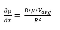
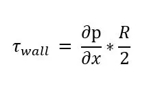
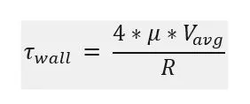
Hagen Poisuelle's equation:

shear stress at the centre is zero as r is zero

velocity variation :

u is zero at walls because of no-slip conditions.

Saving OpenFOAM results in.CSV file using ParaView and analysing with python.

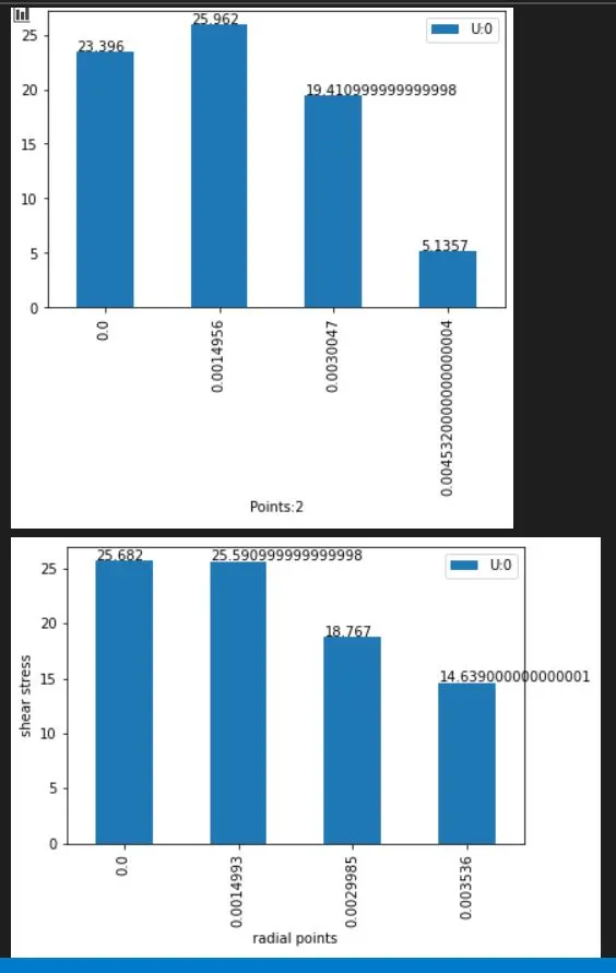
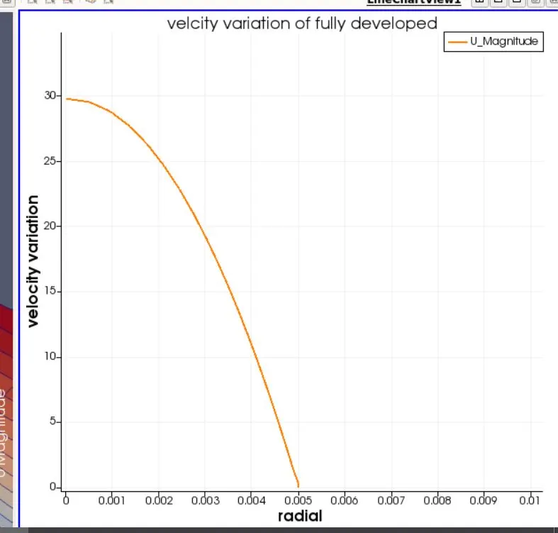
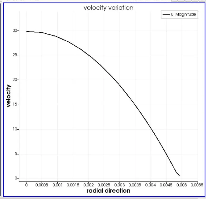
velocity at a radial location	0	0.0015	0.0030	wall
HP	30	27.3	19.2	0
wedge	29.799	27.205	19.177	0.5942
sym10	29.785	27.107	18.3864	0.594
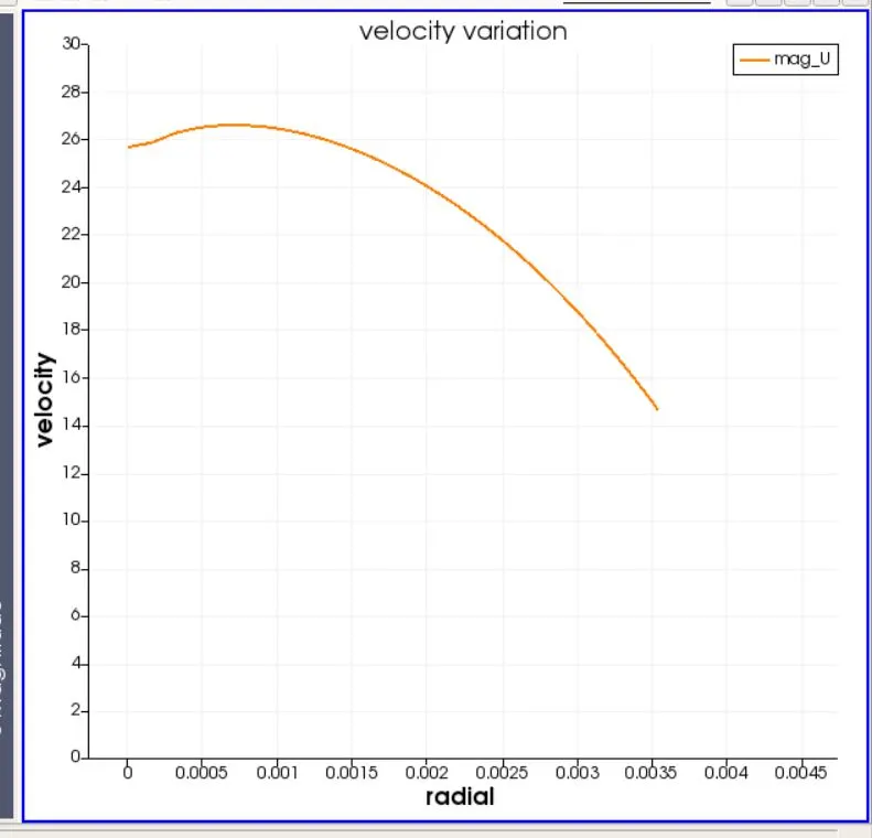
sym25	23.396	25.953	19.379	5.135
sym45	25.682	25.59	18.767	14.639

Python code for data analysis:

import pandas as pd
import matplotlib.pyplot as plt

  
# making data frame from csv file 
df_1 = pd.read_csv(r'G:resultssym10sswed.csv')
df_2 = pd.read_csv(r'G:resultssym10ss10.csv')
df_3 = pd.read_csv(r'G:resultssym10ss25.csv')
df_4 = pd.read_csv(r'G:resultssym10ss45.csv')


# retrieving rows by loc method 
df1 = df_1[df_1['Points:2'].isin([0,0.0014991,0.0029982,0.004997])]
df2 = df_2[df_2['Points:2'].isin([0,0.0015018,0.0029987,0.004924])]
df3 = df_3[df_3['Points:2'].isin([0,0.0014956,0.0030047,0.0045275
])]
df4 = df_4[df_4['Points:2'].isin([0,0.0014993,0.0029985,0.003536])]
#x = dataframe.p
#y = dataframe.arc_length

#ax = df.plot.bar(x, y, rot=0)
#df.plot(x="Points:2", y=["U:0"])
#df.plot.bar(x="Points:2", y=["mag(U)"])

ax_1 = df1.plot.bar(x="Points:2", y=["U:0"])
ax_2 = df2.plot.bar(x="Points:2", y=["U:0"])
ax_3 = df3.plot.bar(x="Points:2", y=["U:0"])
ax_4 = df4.plot.bar(x="Points:2", y=["U:0"])



plt.xlabel ('radial points')
plt.ylabel ('shear stress')
for p in ax_1.patches:

    ax_1.annotate(str(p.get_height()), (p.get_x() * 1.005, p.get_height() * 1.005))
for p in ax_2.patches:

    ax_2.annotate(str(p.get_height()), (p.get_x() * 1.005, p.get_height() * 1.005))
for p in ax_3.patches:

    ax_3.annotate(str(p.get_height()), (p.get_x() * 1.005, p.get_height() * 1.005))
for p in ax_4.patches:

    ax_4.annotate(str(p.get_height()), (p.get_x() * 1.005, p.get_height() * 1.005))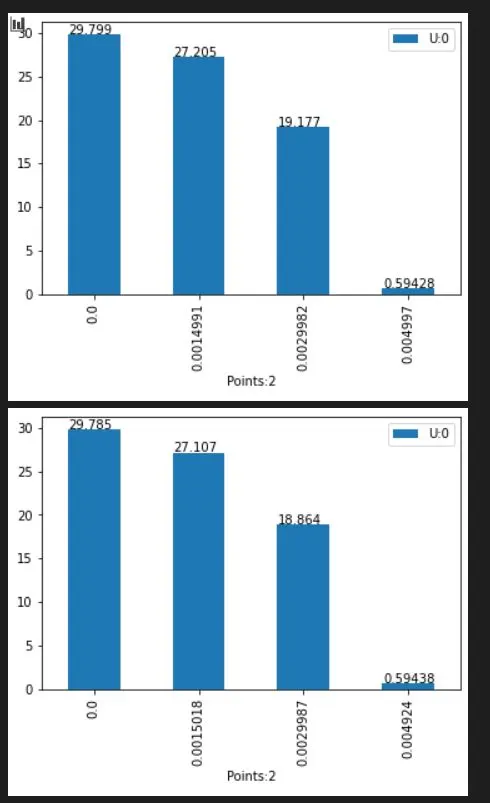

import pandas as pd
import seaborn as sns
import matplotlib.pyplot as plt

  
dataframe_1 = pd.read_csv(r'G:resultssym10sswed.csv')
dataframe_2 = pd.read_csv(r'G:resultssym10ss10.csv')
dataframe_3 = pd.read_csv(r'G:resultssym10ss25.csv')
dataframe_4 = pd.read_csv(r'G:resultssym10ss45.csv')

#ax = df.plot.bar(x, y, rot=0)
#df.plot(x="Points:2", y=["U:0"])
#df.plot.bar(x="Points:2", y=["mag(U)"])

#ax_1 = df_1.plot.bar(x="Points:2", y=["tau:2"])
#ax_2 = df_2.plot.bar(x="Points:2", y=["tau:2"])
dataframe_1['hue']=2.5
dataframe_2['hue']=10
dataframe_3['hue']=25
dataframe_4['hue']=45
res=pd.concat([dataframe_1,dataframe_2,dataframe_3,dataframe_4])
#x = dataframe.Points:2
#y = dataframe.U:0
sns.set_color_codes("dark")
ax = sns.lineplot(x="Points:2", y="U:0",data=res,hue='hue',, palette = "Set1")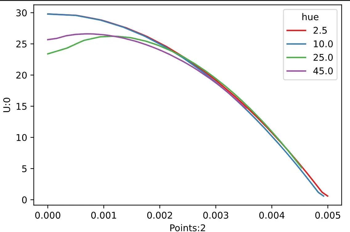

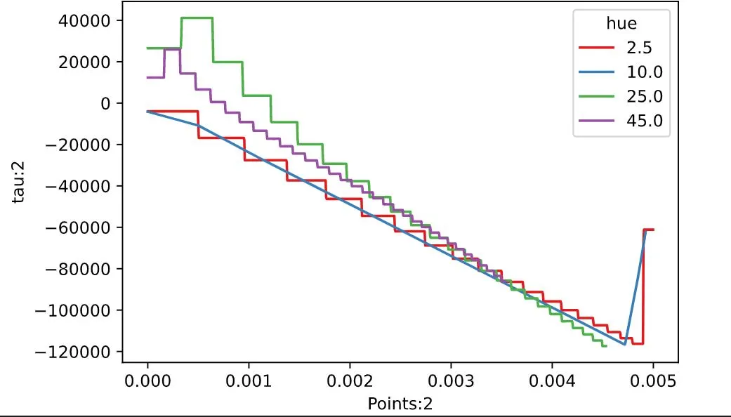
replacing U:0 with tau:2 in same code

wedge

sym10

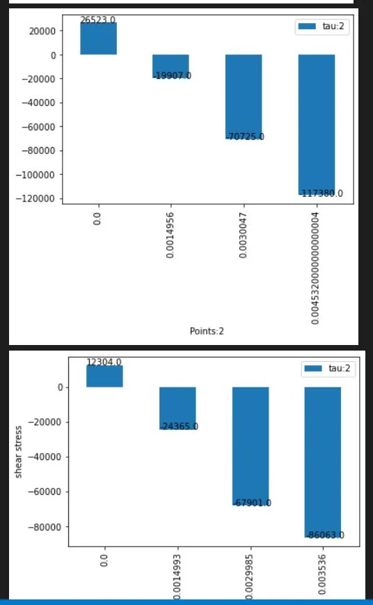
symmetry25:

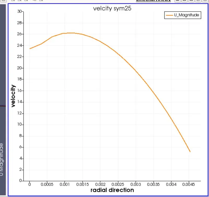
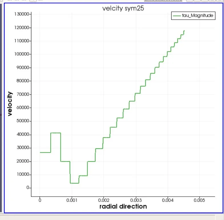
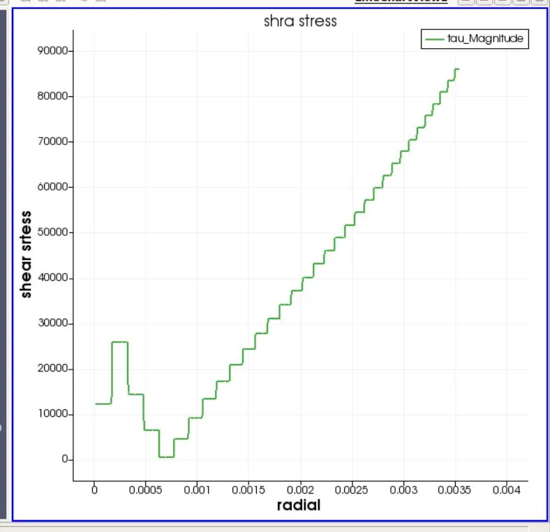
sym 45

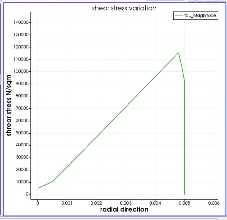
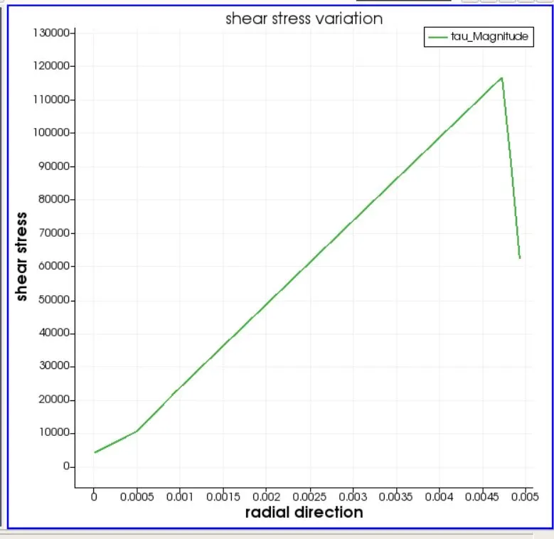
shear stress at a radial location	0	0.0015	0.003	wall
HP	0	-36000	-72000	-119928
wedge	-3981	-37376	-68843	-61143
sym10	-4152	-36469	-73808	-62256
sym25	26523	-19907	-70725	-117380
sym45	12304	-24365	-67901	-86063

Python code for data analysis:

import pandas as pd
import matplotlib.pyplot as plt

  
# making data frame from csv file 
df_1 = pd.read_csv(r'G:resultssym10sswed.csv')
df_2 = pd.read_csv(r'G:resultssym10ss10.csv')
df_3 = pd.read_csv(r'G:resultssym10ss25.csv')
df_4 = pd.read_csv(r'G:resultssym10ss45.csv')


# retrieving rows by loc method 
df1 = df_1[df_1['Points:2'].isin([0,0.0014991,0.0029982,0.004997])]
df2 = df_2[df_2['Points:2'].isin([0,0.0015018,0.0029987,0.004924])]
df3 = df_3[df_3['Points:2'].isin([0,0.0014956,0.0030047,0.0045275
])]
df4 = df_4[df_4['Points:2'].isin([0,0.0014993,0.0029985,0.003536])]

#x = dataframe.p
#y = dataframe.arc_length

#ax = df.plot.bar(x, y, rot=0)
#df.plot(x="Points:2", y=["U:0"])
#df.plot.bar(x="Points:2", y=["mag(U)"])

ax_1 = df1.plot.bar(x="Points:2", y=["tau:2"])
ax_2 = df2.plot.bar(x="Points:2", y=["tau:2"])
ax_3 = df3.plot.bar(x="Points:2", y=["tau:2"])
ax_4 = df4.plot.bar(x="Points:2", y=["tau:2"])



plt.xlabel ('radial points')
plt.ylabel ('shear stress')
for p in ax_1.patches:

    ax_1.annotate(str(p.get_height()), (p.get_x() * 1.005, p.get_height() * 1.005))
for p in ax_2.patches:

    ax_2.annotate(str(p.get_height()), (p.get_x() * 1.005, p.get_height() * 1.005))
for p in ax_3.patches:

    ax_3.annotate(str(p.get_height()), (p.get_x() * 1.005, p.get_height() * 1.005))
for p in ax_4.patches:

    ax_4.annotate(str(p.get_height()), (p.get_x() * 1.005, p.get_height() * 1.005))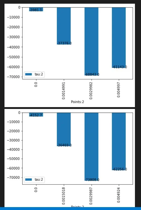

Compare the above results:

1. when we compare velocity results of wedge and symmetry 10 we get almost correct results which compare with HP equations.

2. But for symmetry 25 and 45 results have large errors in velocity which can be observed in table, graph and bar plot also.

3. when we compare shear stress results of wedge and symmetry 10 we get almost correct results except for the wall which compares with HP equations.

4. Wall shear stress or maximum shear stress in wedge and symmetry 10 occurs just before the wall and decreases at the wall as in the graphs which introduces error.

5. But for symmetry 25 and 45 results have large errors in shear stress which can be observed in the table, graph and bar plot also.