Simulation of Flow through a pipe in OpenFoam - Part 1
Simulation of Flow through a pipe in OpenFoam
Internal flow
The flow of liquid or gas through pipes or ducts is commonly used in heating and cooling applications and fluid distribution networks. The fluid in such applications is usually forced to flow by a fan or pump through a flow section. We pay particular attention to friction, which is directly related to the pressure drop and head loss during flow through pipes and ducts. The pressure drop is then used to determine the pumping power requirement. A typical piping system involves pipes of different diameters connected to each other by various fittings or elbows to route the fluid, valves to control the flow rate, and pumps to pressurize the fluid. The terms pipe, duct, and conduit are usually used interchangeably for flow sections. In general, flow sections of the circular cross-section are referred to as pipes (especially when the fluid is a liquid) and flow sections of the noncircular cross-section as ducts (especially when the fluid is a gas). Small-diameter pipes are usually referred to as tubes.
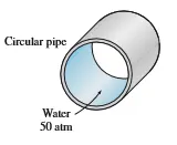
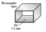
Fluids, especially liquids, are transported in circular pipes. This is because pipes with a circular cross-section can withstand large pressure differences between the inside and the outside without undergoing significant distortion. Noncircular pipes are usually used in applications such as the heating and cooling systems of buildings where the pressure difference is relatively small, the manufacturing and installation costs are lower, and the available space is limited for ductwork.
The fluid velocity in a pipe changes from zero at the wall because of the no-slip condition to a maximum at the pipe center. In fluid flow, it is convenient to work with an average velocity Vavg, which remains constant in incompressible flow when the cross-sectional area of the pipe is constant.
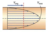
Average velocity Vavg is defined as the average speed through a cross-section. For fully developed laminar pipe flow, Vavg is half of the maximum velocity.
The average velocity for incompressible flow in a circular pipe of radius R is expressed as
Vavg = ∫Ac ρu(r) dAc ρAc = ∫ρu(r)2𝜋r dr ρ𝜋R2 = 2 R2 ∫u(r)r dr (0 to R)
Laminar and Turbulent Flow
The flow in a pipe is streamlined at low velocities but turns chaotic as velocity is increased above a critical value.
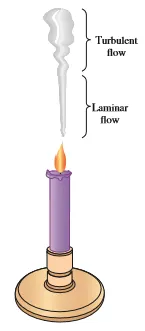
The flow regime in the first case is said to be laminar, characterized by smooth streamlines and highly ordered motion, and turbulent in the second case, where it is characterized by velocity fluctuations and highly disordered motion. The transition from laminar to turbulent flow does not occur suddenly; rather, it occurs over some region in which the flow fluctuates between laminar and turbulent flows before it becomes fully turbulent. Most flows encountered in practice are turbulent. Laminar flow is encountered when highly viscous fluids such as oils flow in small pipes or narrow
passages.
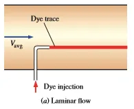
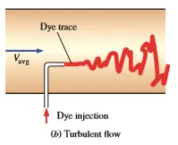
We observe that the dye streak forms a straight and smooth line at low velocities when the flow is laminar (we may see some blurring because of molecular diffusion), has bursts of fluctuations in the transitional regime, and zigzags rapidly and disorderly when the flow becomes fully turbulent. These zigzags and the dispersion of the dye are indicative of the fluctuations in the main flow and the rapid mixing of fluid particles from adjacent layers.
Reynolds Number
The transition from laminar to turbulent flow depends on the geometry, surface roughness, flow velocity, surface temperature, and type of fluid, among other things. After exhaustive experiments in the 1880s, Osborne Reynolds discovered that the flow regime depends mainly on the ratio of inertial forces to viscous forces in the fluid. This ratio is called the Reynolds number and is expressed for internal flow in a circular pipe as
Re = Inertial forces /Viscous forces = VavgD/𝜈 = ρVavgD/𝜇
where Vavg = average flow velocity (m/s), D = characteristic length of the geometry (diameter in this case, in m), and 𝜈 = 𝜇/𝜌 = kinematic viscosity of the fluid (m2/s).
Reynolds number is a dimensionless quantity.
At large Reynolds numbers, the inertial forces, which are proportional to the fluid density and the square of the fluid velocity, are large relative to the viscous forces, and thus the viscous forces cannot prevent the random and rapid fluctuations of the fluid. Small or moderate Reynolds numbers, however, the viscous forces are large enough to suppress these fluctuations and to keep the fluid “in line.” Thus the flow is turbulent in the first case and laminar in the second. The Reynolds number at which the flow becomes turbulent is called the critical Reynolds number, Recr. The value of the critical Reynolds number is different for different geometries and flow conditions. For internal flow in a circular pipe, the generally accepted value of the critical Reynolds number is Recr = 2300.
For flow-through non-circular pipes, the Reynolds number is based on the hydraulic diameter Dh.
Entrance Length
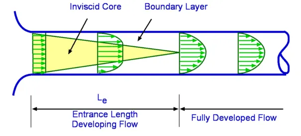
Consider a flow entering a pipe. Let us think of the entering flow being uniform, so inviscid. As soon as the flow 'hits' the pipe many changes take place. The most important of these is that viscosity imposes itself on the flow and the "No Slip" condition at the wall of the pipe comes into effect. Consequently the velocity components are each zero on the wall, ie., u = v = 0. The flow adjacent to the wall decelerates continuously. We have a layer close to the body where the velocity builds up slowly from zero at the wall to a uniform velocity towards the center of the pipe. This layer is what is called the Boundary Layer. Viscous effects are dominant within the boundary layer. Outside of this layer is the inviscid core where viscous effects are negligible or absent.
The boundary layer is not a static phenomenon; it is dynamic. it grows meaning that its thickness increases as we move downstream. From Fig. it is seen that the boundary layer from the walls grows to such an extent that they all merge on the centreline of the pipe. Once this takes place, the inviscid core terminates and the flow is all viscus. The flow is now called a Fully Developed Flow. The velocity profile becomes parabolic. Once the flow is fully developed the velocity profile does not vary in the flow direction. In fact, in this region, the pressure gradient and the shear stress in the flow are in balance. The length of the pipe between the start and the point where the fully developed flow begins is called the Entrance Length. Denoted by Le, the entrance length is a function of the Reynolds Number of the flow. In general,
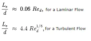
At critical condition, i.e., Red =2300, the Le/d for a laminar flow is 138. Under turbulent conditions it ranges from 18(at Red = 4000) to 95 (at Red=108)
The application decides whether a long enough entrance length is required or a shorter one is required. Take wind tunnel for instance. Here the aim is to have a uniform flow over the model in the test section. So one desires to have a longer entrance length.
Hydrodynamic Entrance Length
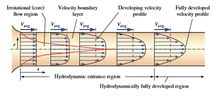
The region from the pipe inlet to the point at which the velocity profile is fully developed is called the hydrodynamic entrance region, and the length of this region is called the hydrodynamic entry length Lh. Flow in the entrance region is called hydrodynamically developing flow since this is the region where the velocity profile develops. The region beyond the entrance region in which the velocity profile is fully developed and remains unchanged is called the hydrodynamically fully developed region. The flow is said to be fully developed when the normalized temperature profile remains unchanged as well. Hydrodynamically fully developed flow is equivalent to fully developed flow when the fluid in the pipe is not heated or cooled since the fluid temperature in this case remains essentially constant throughout. The velocity profile in the fully developed region is parabolic in laminar flow and much flatter (or fuller) in turbulent flow due to eddy motion and more vigorous mixing in the radial direction.
Hagen-Poiseuille's Law
In nonideal fluid dynamics the Hagen–Poiseuille equation, also known as the Hagen–Poiseuille law, Poiseuille law, or Poiseuille equation, is a physical law that gives the pressure drop in an incompressible and Newtonian fluid in laminar flow flowing through a long cylindrical pipe of constant cross-section.
Formulas
Average velocity `V_(avg)=(Re*mu)/(rho*D)`
Maximum velocity `V_(max) = 2*V_(avg)`
Pressure difference `DeltaP = (8*mu*L*V_(avg) )/(r^2)`
Kinematic pressure difference `DeltaP_k=(DeltaP)/rho`
Shrea stress `tau=(2*mu*V_(max)*R)/r^2`
Assumptions:
Diameter D = 0.02
Radius r = 0.01
Dynamic viscosity mu = 0.00089 N/m^2
density rho = 997 kg/m^3
Reynold's Number Re = 2100
Entry length of pipe L = 0.06*Re*D
Total length of pipe L_p = L+0.3
Wedge angle theta = 3
MATLAB coding
Creating blockMeshDict file
% Simulation of flow through a pipe using OpenFoam
% Creating blockMeshDict file

clear all
close all
clc

% Defining variables and assumptions
% Diameter of pipe
D = 0.02;

% Radius
r =D/2;

% Dynamic viscosity N/m^2
mu = 0.00089;

% Density of fluid kg/m^3
rho = 997;

% Reynold's Number for laminar flow
Re = 2100;

% Entry length of pipe
L = 0.06*Re*D;

% Total lenghth of pipe
L_p = L+0.3;

% Wedge angle (less than 5 degree)
theta = 3;

% Hagen Poiseuill's law

% Average velocity
V_avg = (Re*mu)/(rho*D);

% Maximum velocity
V_max = 2*V_avg;

% Pressure difference
del_P = (8*mu*L*V_avg)/(r^2);

% Kinematic pressure difference
K_P = del_P/rho;

% Radial distance
R = linspace(0,r,1000);
% Calculating shear stress (wall shear stress)
for i = 1:length(R)
    tau = (2*mu*V_max*R)/(r^2);
end

% Now creating blockMeshDict file for OpenFoam to generate the geometry

% Adding headers
header1 = '/*--------------------------------*- C++ -*----------------------------------*';
header2 = '  =========                 |';
header3 = '  \      /  F ield         | OpenFOAM: The Open Source CFD Toolbox';
header4 = '   \    /   O peration     | Website:  https://openfoam.org';
header5 = '    \  /    A nd           | Version:  8';
header6 = '     \/     M anipulation  |';
header7 = '*---------------------------------------------------------------------------*/';
header8 = '// * * * * * * * * * * * * * * * * * * * * * * * * * * * * * * * * * * * * * //';
header9 = '// ************************************************************************* //';
% Creating vertices
v0 = [0 0 0]; %point 0
v1 = [ 0 r*cosd(theta/2) -r*sind(theta/2)]; %point 1
v2 = [ 0 r*cosd(theta/2) r*sind(theta/2)]; %point 2
v3 = [L_p 0 0]; %point 3
v4 = [L_p r*cosd(theta/2) -r*sind(theta/2)]; %point 4
v5 = [L_p r*cosd(theta/2) r*sind(theta/2)]; %point 5

% Creating file and writing
f1 = fopen('blockMeshDict','w')

fprintf(f1, '%sn', header1)
fprintf(f1, '%sn', header2)
fprintf(f1, '%sn', header3)
fprintf(f1, '%sn', header4)
fprintf(f1, '%sn', header5)
fprintf(f1, '%sn', header6)
fprintf(f1, '%sn', header7)

fprintf(f1, 'FoamFilen{n')
fprintf(f1, '%12s t 2.0;n','version')
fprintf(f1, '%12s t ascii;n','format')
fprintf(f1, '%12s t dictionary;n','class')
fprintf(f1, '%12s t blockMeshDict','object')
fprintf(f1, '}n')
fprintf(f1, '%snn', header8)

fprintf(f1,'%s 1;nn','covertToMeters')

% Creating vertices
fprintf(f1, '%sn','vertices')
fprintf(f1, '(n')
fprintf(f1, 't(%d %d %d)n',v0)
fprintf(f1, 't(%d %d %d)n',v1)
fprintf(f1, 't(%d %d %d)n',v2)
fprintf(f1, 't(%d %d %d)n',v3)
fprintf(f1, 't(%d %d %d)n',v4)
fprintf(f1, 't(%d %d %d)n',v5)
fprintf(f1, '%2snn',');')

% Creating blocks
fprintf(f1, 'blocksn(n')

% Simple grading factor
grading = 0.2;
% Number of cells
b1 = 50;
b2 = 1;
b3 = 200;
fprintf(f1, 't %s (%d %d %d) %s (%d 0 0)n','hex (0 1 2 0 3 4 5 3)',b1,b2,b3,'simpleGrading',grading)
fprintf(f1, ');nn')

% Creating edges
fprintf(f1, '%sn','edges')
fprintf(f1, '(n')
fprintf(f1, 't arc %d %d (%d %d %d)n',1,2,0,r,0)
fprintf(f1, 't arc %d %d (%d %d %d)n',4,5,L_p,r,0)
fprintf(f1, ');nn')

% Creating boundary
fprintf(f1, '%sn','boundary')
fprintf(f1, '(n')
% Inlet
fprintf(f1, 't inlet nt {n')
fprintf(f1, 't   type  patch;nt')
fprintf(f1, 't   facesnt')
fprintf(f1, 't   (nt')
fprintf(f1, 'tt (0 1 2 0)nt')
fprintf(f1, 't   );nt }n')
% Outlet
fprintf(f1, 't outlet nt {n')
fprintf(f1, 't   type  patch;nt')
fprintf(f1, 't   facesnt')
fprintf(f1, 't   (nt')
fprintf(f1, 'tt (3 4 5 3)nt')
fprintf(f1, 't   );nt }n')
% Top
fprintf(f1, 't top nt {n')
fprintf(f1, 't   type  patch;nt')
fprintf(f1, 't   facesnt')
fprintf(f1, 't   (nt')
fprintf(f1, 'tt (1 2 5 4)nt')
fprintf(f1, 't   );nt }n')
% Front
fprintf(f1, 't front nt {n')
fprintf(f1, 't   type  wedge;nt')
fprintf(f1, 't   facesnt')
fprintf(f1, 't   (nt')
fprintf(f1, 'tt (0 3 5 2)nt')
fprintf(f1, 't   );nt }n')
% back
fprintf(f1, 't back nt {n')
fprintf(f1, 't   type  wedge;nt')
fprintf(f1, 't   facesnt')
fprintf(f1, 't   (nt')
fprintf(f1, 'tt (0 3 4 1)nt')
fprintf(f1, 't   );nt }n')

fprintf(f1, 'n);')

% Mergre patch
fprintf(f1, 'n%s','mergePatchPairs')
fprintf(f1, 'n(')
fprintf(f1, 'n);n')

fprintf(f1, 'n%s', header9)
fclose(f1);
blockMeshDict
/*--------------------------------*- C++ -*----------------------------------*
  =========                 |
  \      /  F ield         | OpenFOAM: The Open Source CFD Toolbox
   \    /   O peration     | Website:  https://openfoam.org
    \  /    A nd           | Version:  8
     \/     M anipulation  |
*---------------------------------------------------------------------------*/
FoamFile
{
     version 	 2.0;
      format 	 ascii;
       class 	 dictionary;
      object 	 blockMeshDict}
// * * * * * * * * * * * * * * * * * * * * * * * * * * * * * * * * * * * * * //

covertToMeters 1;

vertices
(
	(0 0 0)
	(0 9.996573e-03 -2.617695e-04)
	(0 9.996573e-03 2.617695e-04)
	(2.820000e+00 0 0)
	(2.820000e+00 9.996573e-03 -2.617695e-04)
	(2.820000e+00 9.996573e-03 2.617695e-04)
);

blocks
(
	 hex (0 1 2 0 3 4 5 3) (50 1 200) simpleGrading (2.000000e-01 0 0)
);

edges
(
	 arc 1 2 (0 1.000000e-02 0)
	 arc 4 5 (2.820000e+00 1.000000e-02 0)
);

boundary
(
	 inlet
	 {
	   type  patch;
		   faces
		   (
			 (0 1 2 0)
		   );
	 }
	 outlet
	 {
	   type  patch;
		   faces
		   (
			 (3 4 5 3)
		   );
	 }
	 top
	 {
	   type  patch;
		   faces
		   (
			 (1 2 5 4)
		   );
	 }
	 front
	 {
	   type  wedge;
		   faces
		   (
			 (0 3 5 2)
		   );
	 }
	 back
	 {
	   type  wedge;
		   faces
		   (
			 (0 3 4 1)
		   );
	 }

);
mergePatchPairs
(
);

// ************************************************************************* //
Velocity boundary condition
/*--------------------------------*- C++ -*----------------------------------*
  =========                 |
  \      /  F ield         | OpenFOAM: The Open Source CFD Toolbox
   \    /   O peration     | Website:  https://openfoam.org
    \  /    A nd           | Version:  8
     \/     M anipulation  |
*---------------------------------------------------------------------------*/
FoamFile
{
    version     2.0;
    format      ascii;
    class       volVectorField;
    object      U;
}
// * * * * * * * * * * * * * * * * * * * * * * * * * * * * * * * * * * * * * //

dimensions      [0 1 -1 0 0 0 0];

internalField   uniform (0.0937312 0 0);

boundaryField
{
    axis
    {
    	type		empty;
    }
    inlet
    {
        type            fixedValue;
        value           uniform (0.0937312 0 0);
    }

    outlet
    {
        type            zeroGradient;
    }

    top
    {
    	type		fixedValue;
    	value		uniform (0 0 0);
    }

    front
    {
        type            wedge;
    }
    back
    {
        type            wedge;
    }
}

// ************************************************************************* //
Pressure boundary condition
/*--------------------------------*- C++ -*----------------------------------*
  =========                 |
  \      /  F ield         | OpenFOAM: The Open Source CFD Toolbox
   \    /   O peration     | Website:  https://openfoam.org
    \  /    A nd           | Version:  8
     \/     M anipulation  |
*---------------------------------------------------------------------------*/
FoamFile
{
    version     2.0;
    format      ascii;
    class       volScalarField;
    object      p;
}
// * * * * * * * * * * * * * * * * * * * * * * * * * * * * * * * * * * * * * //

dimensions      [0 2 -2 0 0 0 0];

internalField   uniform 0;

boundaryField
{
    axis
    {
    	type		empty;
    }
    inlet
    {
        type            zeroGradient;
    }

    outlet
    {
        type            fixedValue;
        value           uniform 0.018;
    }

    top
    {
    	type		zeroGradient;
    }

    front
    {
        type            wedge;
    }
    back
    {
        type            wedge;
    }
}

// ************************************************************************* //
Transport property
/*--------------------------------*- C++ -*----------------------------------*
  =========                 |
  \      /  F ield         | OpenFOAM: The Open Source CFD Toolbox
   \    /   O peration     | Website:  https://openfoam.org
    \  /    A nd           | Version:  8
     \/     M anipulation  |
*---------------------------------------------------------------------------*/
FoamFile
{
    version     2.0;
    format      ascii;
    class       dictionary;
    location    "constant";
    object      transportProperties;
}
// * * * * * * * * * * * * * * * * * * * * * * * * * * * * * * * * * * * * * //

nu              [0 2 -1 0 0 0 0] 1e-06;


// ************************************************************************* //
controlDict
/*--------------------------------*- C++ -*----------------------------------*
  =========                 |
  \      /  F ield         | OpenFOAM: The Open Source CFD Toolbox
   \    /   O peration     | Website:  https://openfoam.org
    \  /    A nd           | Version:  8
     \/     M anipulation  |
*---------------------------------------------------------------------------*/
FoamFile
{
    version     2.0;
    format      ascii;
    class       dictionary;
    location    "system";
    object      controlDict;
}
// * * * * * * * * * * * * * * * * * * * * * * * * * * * * * * * * * * * * * //

application     icoFoam;

startFrom       startTime;

startTime       0;

stopAt          endTime;

endTime         50;

deltaT          0.01;

writeControl    timeStep;

writeInterval   200;

purgeWrite      0;

writeFormat     ascii;

writePrecision  6;

writeCompression off;

timeFormat      general;

timePrecision   6;

runTimeModifiable true;


// ************************************************************************* //
Results:
Profile
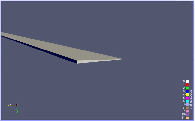
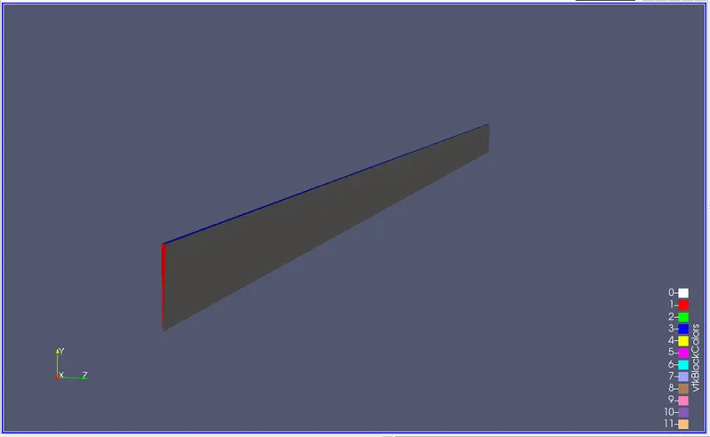
Mesh
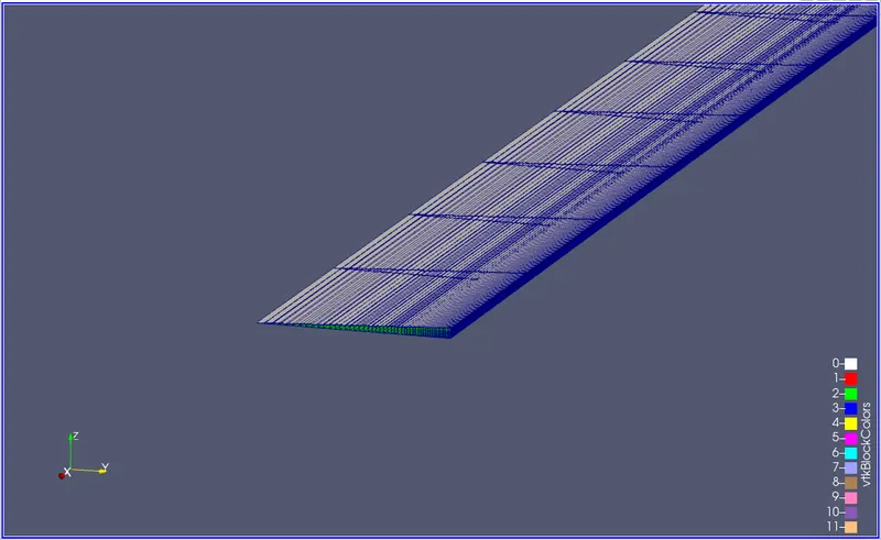
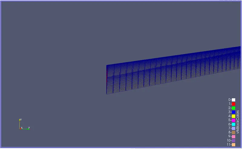
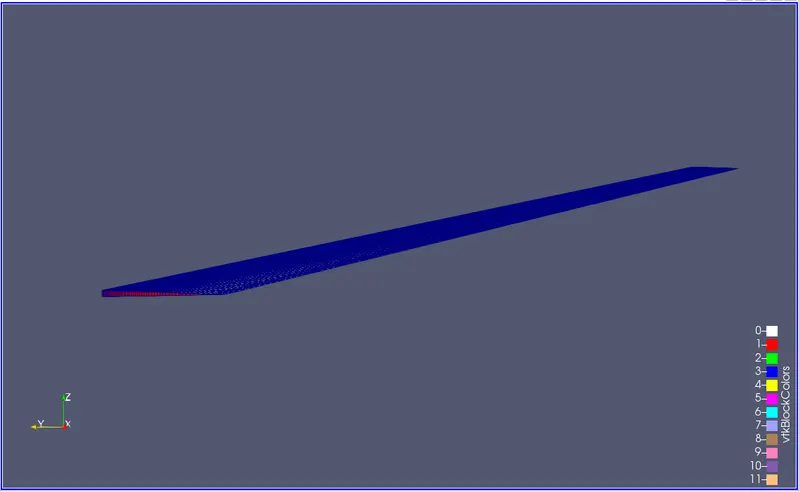
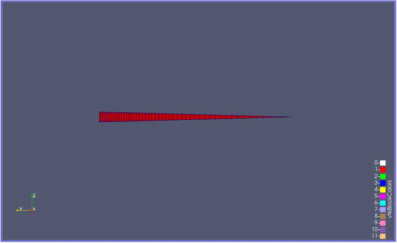
Pressure diagram
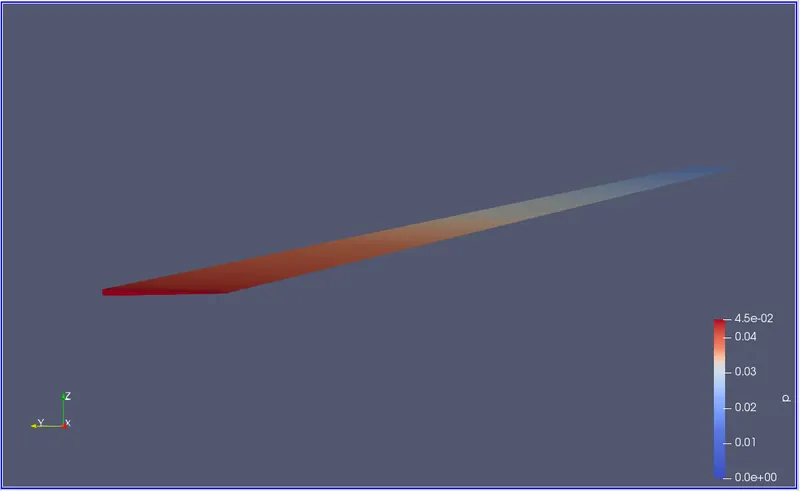
Velocity Diagram
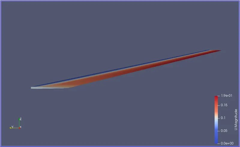
Velocity profile at hydrodynamic entrance length 2.52m
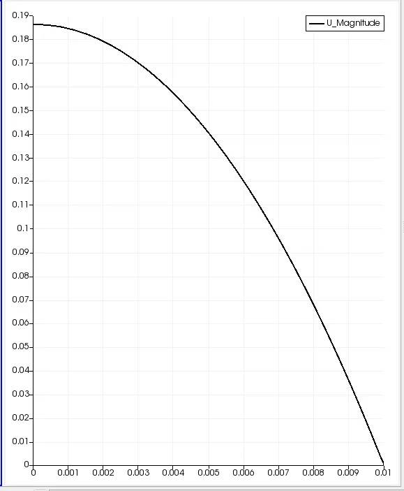
For 0.01m
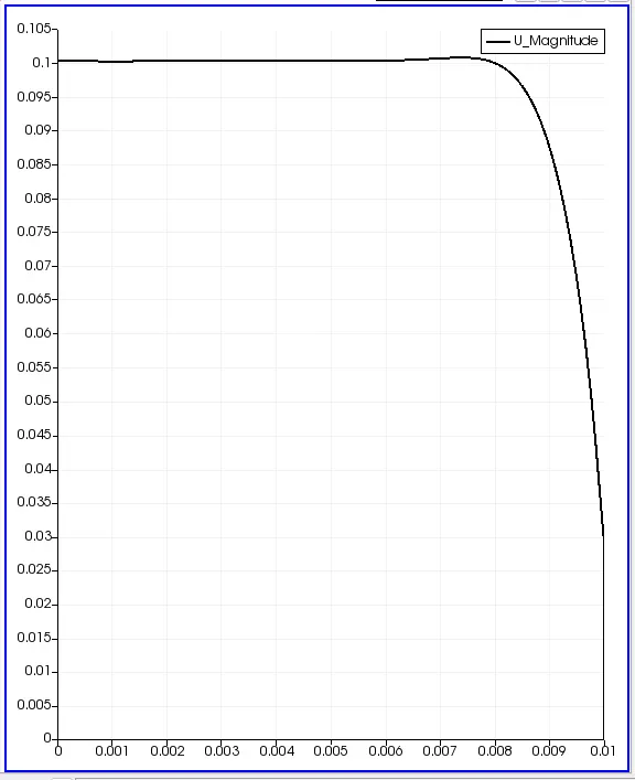
For 0.05m
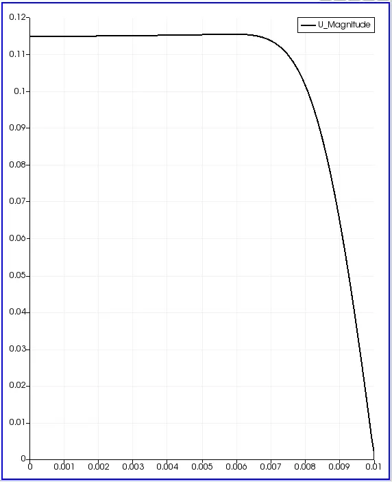
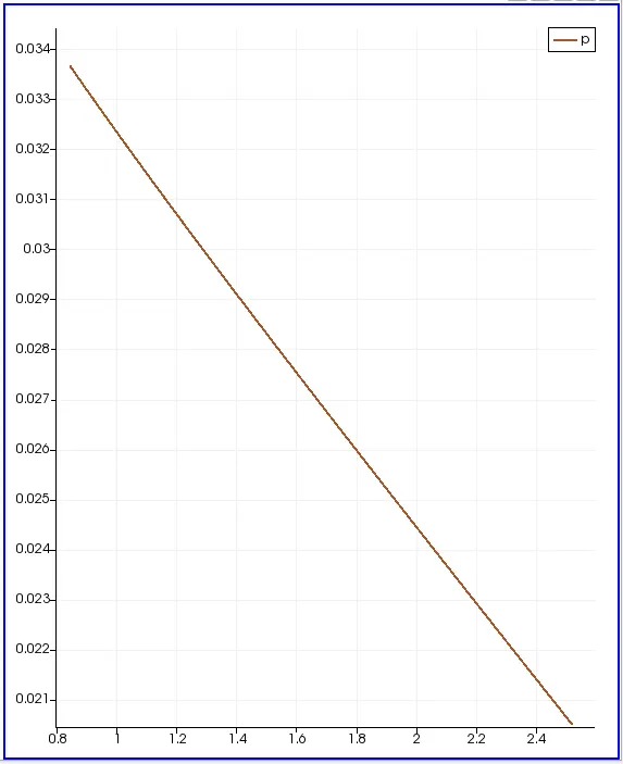
Pressure profile
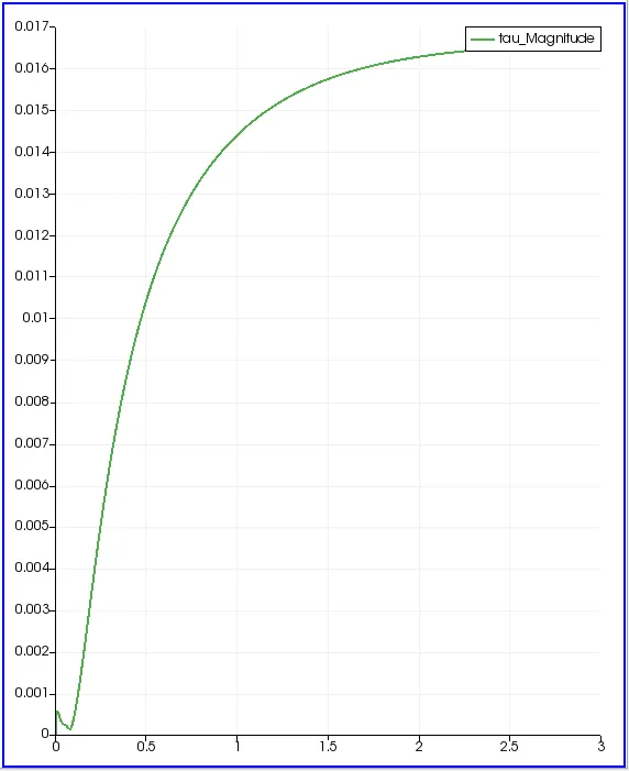
Shear stress
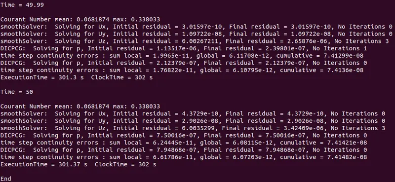
Courant number mean = 0.0681874
Courant number max = 0.338033
Execution time = 301.37 sec
Clock time = 302 sec
Comparing results:
| Wedge angle | Maximum velocity (analytical) | Maximum velocity (Hagen-Poiseuille) |
| 3 | 18.80 | 18.75 |
| 4 | 18.83 | 18.75 |
| Error | 0.03 | 0.00 |