Week 11 - Simulation of Flow through a pipe in OpenFoam
Simulation of flow through the pipe in open Foam:
The objective of the challenge is to perform a simulation of flow through the pipe using the Open Foam tool. Here we have taken a wedge-shaped body to perform the simulation. A proper code has to be written in the block-Dict file to get the desired shape. The fluid used in the simulation is water at room temperature. The Flow is laminar in nature. For this condition, we use the icoFoam solver in OpenFoam to solve the case.
Hagen-Poiseuille Flow
The Hagen-Poiseuille Flow is a type of fluid flow based on the Hagen-Poiseuille Law, which is a physical law that gives the pressure drop in an incompressible and Newtonian fluid in laminar flow flowing through a long cylindrical pipe of constant cross-section. Hagen-Poiseuille Flow or simply Poiseuille Flow is the guiding principle behind a variety of applications like airflow through the lung alveoli, fluid flow through a drinking straw or through a hypodermic needle. In essence, Poiseuille's Equation is used to describe the pressure drop due to the viscosity of the fluid.
The assumption of the HP Equation is that the fluid is incompressible and Newtonian, and the flow is laminar through a pipe of constant cross-section, with a length that is sufficiently larger than the diameter of the pipe, and that there is no acceleration of the fluid through the pipe.
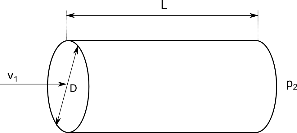
Consider a Cylindrical pipe of circular cross-section as shown above. Let the diameter of the pipe be D and the Length of the Pipe be L. Assume a fluid flowing through the pipe with an inlet velocity of v1 and let pressure at the outlet of the pipe be p2. For this project, the diameter of the pipe is assumed to be 0.02m or 20mm, and the length of the pipe is taken as 3m. The length of the pipe has been decided based on the Hydrodynamic Entrance Length (Le) obtained, which will be explained in upcoming sections. Let water be the working fluid flowing through the pipe. Thus, the characteristic properties of water such as density (`rho`) and viscosity (`mu`) are taken into account to simulate the fluid flow. Since Hagen-Poiseuille Flow is laminar flow, Reynold's Number pertaining to the Laminar Flow regime (Re = 2100) is considered to simulate the fluid flow and calculate the fluid velocity. In order to minimize the computational resources required for simulating the problem, a section of the pipe or a wedge with a specific wedge angle (less than 5 degrees) is considered, and the symmetry boundary conditions are applied. Considering the aforementioned input values, a MATLAB Script is created to automate the generation of the computational mesh using blockMeshDict to be used in OpenFOAM.
Entrance length:
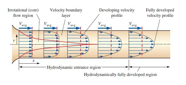
The length of the entrance is the distance that fluid travels after entering a pipe before the full development of the flow. Entrance length refers to the length of the entry region, where effects from the pipe's interior wall spread as an expanding boundary layer into the flow. When the boundary layer extends to fill the entire pipe, the flow grows into a fully developed flow where the flow characteristics no longer change with increased distance along the pipe. To define a variety of flow conditions, there are many different entrance lengths.
Hydrodynamic entrance length:
The hydrodynamic entrance region refers to the area of a pipe where fluid entering a pipe develops a velocity profile due to viscous forces spreading from a pipe's interior wall. This region has a non-uniform flow. The fluid enters a pipe at a constant speed, so fluid particles in the layer in contact with the pipe's surface come to a complete stop because of the no-slip rule. The layer in contact with the pipe surface is resistant to the acceleration of neighboring layers due to viscous forces within the fluid and slowly slows down adjacent layers of fluid, creating a velocity profile. To keep the mass true, the speed of the fluid layers in the center of the pipe increases to compensate for the reduced speed of the fluid layers near the surface of the pipe. It creates a gradient of velocity across the pipe cross-section.
Entry length for the laminar flow is
`L_e =0.06 times R_e timesD`
Entry length for the laminar flow is
`L_e =4.4 times R_e^0.166 times D`
To do the simulation we need to find properties using some variables. Those are Hagen Poiseuille equations.
Variables :
Diameter ,D = 0.004
Radius, r = 0.002
Radial Distance, R = 0 to r
Dynamic viscosity, mu = 0.00089 N/m^2
Density, rho = 997 kg/m^3
Reyonlds number, Re =2100
Hagen–Poiseuille equation
In nonideal fluid dynamic, the Hagen–Poiseuille equation, also known as the Hagen–Poiseuille law, Poiseuille law or Poiseuille equation, is a physical law that gives the pressure drop in an incompressible and Newtonian fluid in laminar flow flowing through a long cylindrical pipe of constant cross section.
Formulaes
Avaerage velocity - `V_(avg) = (R_e times mu)/(rho times D)`
Maximum Velocity - `V_(max) = 2 times V_(avg)`
Pressure difference - `DeltaP =(8 times mu times L times V_(avg))/r^2`
Kinematic Pressure difference - `DeltaP_k = (DeltaP)/rho`
Shear Stress - `tau = (2 times mu times V_(max) times R)/r^2`
Program:
- In the task of generating the blockMeshDict file which generates the mesh file in the OpenFOAM tool for that, we need to write code.
- We also included the codes producing the analytical solution for the fluid v avg, v max, pressure difference, kinematic pressure-difference, and shear stress.
blockMeshDict
/*--------------------------------*- C++ -*----------------------------------*\
  =========                 |
  \\      /  F ield         | OpenFOAM: The Open Source CFD Toolbox
   \\    /   O peration     | Website:  https://openfoam.org
    \\  /    A nd           | Version:  7
     \\/     M anipulation  |
\*---------------------------------------------------------------------------*/
FoamFile
{
    version     2.0;
    format      ascii;
    class       dictionary;
    object      blockMeshDict;
}
// * * * * * * * * * * * * * * * * * * * * * * * * * * * * * * * * * * * * * //

convertToMeters 1;

vertices
(
	 (0  0 0)
	 (0  1.998782e-03 6.979899e-05)
	 (0  1.998782e-03 -6.979899e-05)
	 (1.204000e+00  0 0)
	 (1.204000e+00  1.998782e-03 6.979899e-05)
	 (1.204000e+00  1.998782e-03 -6.979899e-05)
);

blocks
(
	 hex (0 3 5 2 0 3 4 1) (300 30 1) SimpleGrading (1 0.1 1)

);

edges
(
	 arc 1 2 (0 2.000000e-03 0)
	 arc 4 5 (1.204000e+00 2.000000e-03 0)
);

boundary
(
	 inlet
	 {
		 type patch;
		 faces
		 (
			 (0 1 2 0)
		 );
	 }
	 outlet
	 {
		 type patch;
		 faces
		 (
			 (3 5 4 3)
		 );
	 }
	 top
	 {
		 type wall;
		 faces
		 (
			 (1 4 5 2)
		 );
	 }
	 front
	 {
		 type wedge;
		 faces
		 (
			 (0 3 4 1)
		 );
	 }
	 back
	 {
		 type wedge;
		 faces
		 (
			 (0 2 5 3)
		 );
	 }
	 axis
	 {
		 type empty;
		 faces
		 (
			 (0 3 3 0)
		 );
	 }
);

mergePatchPairs
(
);
// * * * * * * * * * * * * * * * * * * * * * * * * * * * * * * * * * * * * * //
controlDict
/*--------------------------------*- C++ -*----------------------------------*\
  =========                 |
  \\      /  F ield         | OpenFOAM: The Open Source CFD Toolbox
   \\    /   O peration     | Website:  https://openfoam.org
    \\  /    A nd           | Version:  7
     \\/     M anipulation  |
\*---------------------------------------------------------------------------*/
FoamFile
{
    version     2.0;
    format      ascii;
    class       dictionary;
    location    "system";
    object      controlDict;
}
// * * * * * * * * * * * * * * * * * * * * * * * * * * * * * * * * * * * * * //

application     icoFoam;

startFrom       startTime;

startTime       0;

stopAt          endTime;

endTime         1;

deltaT          0.001;

writeControl    timeStep;

writeInterval   20;

purgeWrite      0;

writeFormat     ascii;

writePrecision  6;

writeCompression off;

timeFormat      general;

timePrecision   6;

runTimeModifiable true;


// ************************************************************************* //
Pressure
/*--------------------------------*- C++ -*----------------------------------*\
  =========                 |
  \\      /  F ield         | OpenFOAM: The Open Source CFD Toolbox
   \\    /   O peration     | Website:  https://openfoam.org
    \\  /    A nd           | Version:  7
     \\/     M anipulation  |
\*---------------------------------------------------------------------------*/
FoamFile
{
    version     2.0;
    format      ascii;
    class       volScalarField;
    object      p;
}
// * * * * * * * * * * * * * * * * * * * * * * * * * * * * * * * * * * * * * //

dimensions      [0 2 -2 0 0 0 0];

internalField   uniform 0;

boundaryField
{
    inlet
    {
        type            zeroGradient;
    }

    outlet
    {
        type            fixedValue;
       value uniform 1.0073;
    }

    axis
    {
        type            empty;
    }

    top
    {
        type            zeroGradient;
    }

    front
    {
        type            wedge;
    }

    back
    {
        type            wedge;
    }

}

// ************************************************************************* //
Velocity
/*--------------------------------*- C++ -*----------------------------------*\
  =========                 |
  \\      /  F ield         | OpenFOAM: The Open Source CFD Toolbox
   \\    /   O peration     | Website:  https://openfoam.org
    \\  /    A nd           | Version:  7
     \\/     M anipulation  |
\*---------------------------------------------------------------------------*/
FoamFile
{
    version     2.0;
    format      ascii;
    class       volVectorField;
    object      U;
}
// * * * * * * * * * * * * * * * * * * * * * * * * * * * * * * * * * * * * * //

dimensions      [0 1 -1 0 0 0 0];

internalField   uniform (0.4686 0 0);

boundaryField
{
    inlet
    {
       type             fixedValue;
       value uniform (0.4686 0 0);
    }

    outlet
    {
        type            zeroGradient;
    }

    axis
    {
        type            empty;
    }

    top
    {
       type             fixedValue;
       value uniform (0 0 0);
    }

    front
    {
        type            wedge;
    }

    back
    {
        type            wedge;
    }

}

// ************************************************************************* //
Transport Properties
/*--------------------------------*- C++ -*----------------------------------*\
  =========                 |
  \\      /  F ield         | OpenFOAM: The Open Source CFD Toolbox
   \\    /   O peration     | Website:  https://openfoam.org
    \\  /    A nd           | Version:  7
     \\/     M anipulation  |
\*---------------------------------------------------------------------------*/
FoamFile
{
    version     2.0;
    format      ascii;
    class       dictionary;
    location    "constant";
    object      transportProperties;
}
// * * * * * * * * * * * * * * * * * * * * * * * * * * * * * * * * * * * * * //

nu              [0 2 -1 0 0 0 0] 0.892e-6;


// ************************************************************************* //
Matlab Code
clear all
close all
clc

% The Reynolds number
Re = 2100
% The Diameter of pipe
D = 0.004
% The Entry length of pipe
L =0.06*Re*D
% The total length of pipe
L_p = L+0.7
% Radius of pipe
r = D/2
% Angle of wedge (less than 5)
theta = 4
% Dynamic viscosity
mu = 0.89e-3
% Density
rho = 997

% Hagen poiseuille flow equations
v_avg = (Re*mu)/(rho*D)
v_max = 2*(v_avg)
del_p = (8*mu*L_p*v_avg)/(r^2)
kinematic_p = del_p/rho

% calculating shear stress
R = linspace(0,(D/2),1000)

for i = 1:length(R)
    tau(i) = 2*mu*v_max*(abs(R(i)))/r^2
end

plot(R,tau)
xlabel('Radius')
ylabel('Shear stress')
grid on
legend ('Shear stress')


header1='/*----------------------------------*- C++ -*------------------------------------*\'
header2='  =========                 |                                                    '
header3='   \\      /  F ield                | OpenFOAM: The Open Source CFD Toolbox      '
header4='    \\    /   O peration        | Website:  https://openfoam.org                 '
header5='     \\  /    A nd                 | Version:  7                                 '
header6='      \\/     M anipulation   |                                                  '
header7='\*----------------------------------------------------------------------------------*/'

f1 = fopen('blockMeshDict','w')
fprintf(f1, '%s\n', header1)
fprintf(f1, '%s\n', header2)
fprintf(f1, '%s\n', header3)
fprintf(f1, '%s\n', header4)
fprintf(f1, '%s\n', header5)
fprintf(f1, '%s\n', header6)
fprintf(f1, '%s\n', header7)

fprintf(f1, 'FoamFile\n{\n')
fprintf(f1, '%12s \t 2.0;\n','version')
fprintf(f1, '%12s \t ascii;\n','format')
fprintf(f1, '%12s \t dictionary;\n','class')
fprintf(f1, '%12s \t blockMeshDict;\n','object')
fprintf(f1, '}\n')
header8='// * * * * * * * * * * * * * * * * * * * * * * * * * * * * * * * * * * * * * //'
fprintf(f1, '%s\n\n',header8)


fprintf(f1, 'convertToMeters 1;\n\n')

fprintf(f1, 'vertices\n')
fprintf(f1, '(\n')
fprintf(f1, '\t (%d  %d %d)\n',0,0,0)
fprintf(f1, '\t (%d  %d %d)\n',0,r*cosd(theta/2),r*sind(theta/2))
fprintf(f1, '\t (%d  %d %d)\n',0,r*cosd(theta/2),-r*sind(theta/2))
fprintf(f1, '\t (%d  %d %d)\n',L_p,0,0)
fprintf(f1, '\t (%d  %d %d)\n',L_p,r*cosd(theta/2),r*sind(theta/2))
fprintf(f1, '\t (%d  %d %d)\n',L_p,r*cosd(theta/2),-r*sind(theta/2))
fprintf(f1, ');\n\n')


fprintf(f1, 'blocks\n')
fprintf(f1, '(\n')
fprintf(f1, '\t hex (0 3 5 2 0 3 4 1) (%d %d %d)',300,30,1)
fprintf(f1, ' SimpleGrading (1 0.1 1)\n\n')
fprintf(f1, ');\n\n')

fprintf(f1, 'edges\n')
fprintf(f1, '(\n')
fprintf(f1, '\t arc %d %d (%d %d %d)\n',1,2,0,r,0)
fprintf(f1, '\t arc %d %d (%d %d %d)\n',4,5,L_p,r,0)
fprintf(f1, ');\n\n')

fprintf(f1, 'boundary\n')
fprintf(f1, '(\n')
fprintf(f1, '\t inlet \n')
fprintf(f1, '\t {\n')
fprintf(f1, '\t\t type patch;\n')
fprintf(f1, '\t\t faces\n')
fprintf(f1, '\t\t (\n')
fprintf(f1, '\t\t\t (0 1 2 0)\n')
fprintf(f1, '\t\t );\n')
fprintf(f1, '\t }\n')


fprintf(f1, '\t outlet\n')
fprintf(f1, '\t {\n')
fprintf(f1, '\t\t type patch;\n')
fprintf(f1, '\t\t faces\n')
fprintf(f1, '\t\t (\n')
fprintf(f1, '\t\t\t (3 5 4 3)\n')
fprintf(f1, '\t\t );\n')
fprintf(f1, '\t }\n')


fprintf(f1, '\t top\n')
fprintf(f1, '\t {\n')
fprintf(f1, '\t\t type wall;\n')
fprintf(f1, '\t\t faces\n')
fprintf(f1, '\t\t (\n')
fprintf(f1, '\t\t\t (1 4 5 2)\n')
fprintf(f1, '\t\t );\n')
fprintf(f1, '\t }\n')

fprintf(f1, '\t front\n')
fprintf(f1, '\t {\n')
fprintf(f1, '\t\t type wedge;\n')
fprintf(f1, '\t\t faces\n')
fprintf(f1, '\t\t (\n')
fprintf(f1, '\t\t\t (0 3 4 1)\n')
fprintf(f1, '\t\t );\n')
fprintf(f1, '\t }\n')

fprintf(f1, '\t back\n')
fprintf(f1, '\t {\n')
fprintf(f1, '\t\t type wedge;\n')
fprintf(f1, '\t\t faces\n')
fprintf(f1, '\t\t (\n')
fprintf(f1, '\t\t\t (0 2 5 3)\n')
fprintf(f1, '\t\t );\n')
fprintf(f1, '\t }\n')

fprintf(f1, '\t axis\n')
fprintf(f1, '\t {\n')
fprintf(f1, '\t\t type empty;\n')
fprintf(f1, '\t\t faces\n')
fprintf(f1, '\t\t (\n')
fprintf(f1, '\t\t\t (0 3 3 0)\n')
fprintf(f1, '\t\t );\n')
fprintf(f1, '\t }\n')
fprintf(f1, '); \n\n')

fprintf(f1, 'mergePatchPairs\n')
fprintf(f1, '(\n')
fprintf(f1, ');\n')

header9='// * * * * * * * * * * * * * * * * * * * * * * * * * * * * * * * * * * * * * //'
fprintf(f1, '%s\n',header9)

fclose(f1)
Stepwise Procedure for creating the geometry file:
Firstly, we need to calculate the average velocity of the given fluid. For that, we need to given inputs of Reynolds number, Diameter, Viscosity, and Density values.
- Give proper header files that can generate the OpenFOAM header. Be very careful with parenthesis like commas, brackets and slash symbols which may lead us to errors.
- Angles for the wedge has been given in the program.
- Using all these values we calculate average Velocity, Maximum Velocity, Pressure Difference, and kinematic Pressure difference. The reason to calculate the kinematic pressure difference is in the OpenFOAM pressure file if we observe the units, units given are kinematic pressure.
- The angle theta taken less than five degrees is because only one line has to pass through the center of the axis of symmetry
- By using the file parsing technique, We need to write the Matlab code that can be useful to perform the simulations using different angles.
- After getting the BlockMesh Dict file, copy it to the case setup file which is located in the run folder.
- Like this, change other parameters like Velocity, Pressure, and Transport properties file which is obtained from the analytical solution means values obtained from the Matlab code.
- Now set the start and end time in the control-Dict file, and Mention the delta T values also.
- Now place the command directory file in the cavity, run the file using command “block-Mesh”.
- The Above command gives us the mesh file.
- Now check the mesh to see whether any error in mesh, Non-alignment and some other using ‘checkMesh’ command.
- Once the mesh check is over and success. Now use ‘icoFoam’ solver to run the case setup.
- After running successfully, Use ‘paraFoam’ command to post-process the velocity and shear stress of the fluid.
Results:
Generated Geometry
Generated Mesh
Wedge angle 4 degree
Generated Results
Velocity Profiles at Various distances
1. Velocity profile at entrance
While observing the velocity profile at the entrance, we can see that velocity is 0.46 and and the flow is about to develop.
2. Velocity profile at 0.01m
Likewise, if we observe plots below the profile slowly becoming in a parabolic form. That means flow is developing slowly.
3. Velocity profile at 0.2m
4. Velocity profile at 0.35m
And in above two plots for length 0.2 and 0.35, the maximum velocity did not obtain. Means at that length flow did not get fully developed.
5. Velocity profile at 0.5m
At the length of 0.504, the flow gets fully developed because of the maximum velocity obtained here. And it can be seen in the plot for the velocity profile at length 0.504. At length 0.504, it is the same length which was calculated by using the entry length formula the flow gets fully developed. From there furtherly flow profile looks similar and unchanged.
For the understanding below velocity profile plots for 0.7m,1m and 1.2m are shown below.
6. Velocity profile at 0.7m
7. Velocity profile at 1m
8. Velocity profile at 1.2m
From the above plots it can be observed that once the flow is developed at 0.504m the velocity profile from there further flow profile remains unchanged.
Comparison for different Wedge angles
|
Hagen Poisuelle's |
2-deg wedge |
3-deg wedge |
4-deg wedge |
|
|
Courant number mean |
- |
0.118433 |
0.118433 | 0.118433 |
|
Courant number max |
- |
0.472037 |
0.472037 |
0.472037 |
|
Clock Time(sec) |
- |
181 |
179 |
178 |
|
U-max (m/sec) |
0.9373 |
0.934408 |
0.934412 |
0.934416 |
Shear stress Graph:
.Shear stress :
1. When the fluid is in motion, shear stresses are developed due to the particles in the fluid moving relative to one another.
2. For a fluid flowing in a pipe Fluid velocity will be zero at the pipe wall. Velocity will increase while moving towards the center of the pipe. Shear Force is normally present because the adjacent layer of the fluid move with different velocities compared to each other.
3. Fluids Obeying Newton's law where the values of “mu” are constant are known as Newtonian fluids. If ‘mu’ is constant, the shear stress is linearly dependent on the velocity gradient.
Analytically :
Shear stress can be calculated by using the below part of the Matlab code which is written to generate the block-Mesh Dict file.
% calculating shear stress
R = linspace(0,(D/2),1000)

for i = 1:length(R)
    tau(i) = 2*mu*v_max*(abs(R(i)))/r^2
end

plot(R,tau)
xlabel('Radius')
ylabel('Shear stress')
grid on
legend ('Shear stress')
Numerically Shear stress is calculated by considering the velocity of this relative motion, the Shear rate can be calculated shear rate is defined as a measurement of the extent or rate of relative motion between the adjacent layer of the moving fluid. The shear rate for fluid flowing between two parallel plates one moving at a constant speed and one is stationary.
Is determined by `gamma = (u/y)`
where, `(u/y)` is a velocity gradient.
Shear stress is proportional to shear rate where viscosity is the proportionality coefficient. This is known as Newton's law of viscosity.
`tau = mu ((du)/(dy))`
- The above expression is valid only for the low range of Reynolds numbers like laminar flows.
- coming to the turbulent flows it doesn’t work because are any well-defined layers. Instead, unsteady vortices appear of many sizes that interact with each other in a rather chaotic manner
- A separate code has to write to calculate the shear stress numerically.
- Before that, we need to extract the velocity values from the OpenFOAM.
- Using a “CSV” file, we can extract all the velocity (`U_(magnitude),U_x,U_y,U_z`) and pressure values. The “.CSV” is more like an Excel sheet, directly we can upload it to Matlab.
- After uploading it into Matlab, Select only “u” (U_magnitude) values and upload it to the workspace.
- After uploading we need to write a Matlab code to calculate the shear stress.
Shear stress code for Numerical solution:
mu = 0.89e-3;
D = 0.004;

% calculating shear stress
R = linspace(0,(D),1000);

dR = R(2)-R(1);

for i = 1:length(R)
    du = u(i+1)-u(i);
    dU = abs(du);
    tau(i) = mu*(dU/dR);
end


plot(R,tau)
xlabel('Radius')
ylabel('Shear stress')
grid on
legend('Shear stress')
After running the code successfully, we obtain the following plot
Shear stress graph:
- If we see the shear stress near the walls is maximum and at the center of the pipe is zero.
- In the graph there are some step kind of profile is observed, but at last, the solution gets converged.
- The results are matched with the analytical solution.
Comparing the results
|
Maximum Values |
Velocity (m/sec) |
Shear Stress (N/m^2) |
|
Analytical Solution |
0.9373 |
0.4222 |
|
Numerical Solution |
0.9253 |
0.4112 |
|
Error % |
1.28 |
2.60 |
The shear stress value is maximum at the pipe wall and minimum at the pipe center, which is in accordance with the experimental findings.