week-11 Joint creation and Demonstration
Assignment 11
1. Part creation
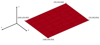
The first part (Deformable body) to be created in LS Dyna was a square surface with a side of 30 mm. The created geometry was meshed with 5mm square elements and translated so that its corner nodes could have the coordinates seen in the figure below.
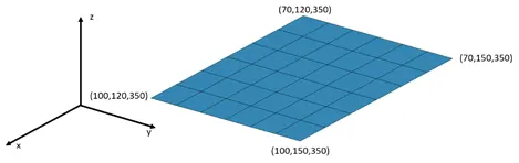
The second part (Rigid body) was created using a similar procedure, and the same type of mesh was used.
|
NID |
X |
Y |
Z |
|
1 |
100 |
120 |
350 |
|
2 |
100 |
120 |
350 |
|
3 |
100 |
150 |
350 |
|
4 |
100 |
150 |
350 |
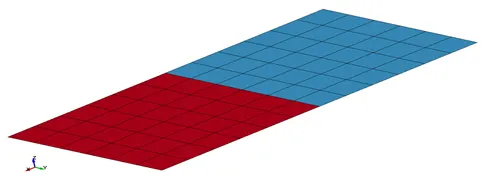
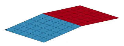
The meshed model is shown in the following figure.
2. Unit system
Before any further definitions of the models, the unit system is defined as follows:
m-Kg-s (IS)
3. Material definition
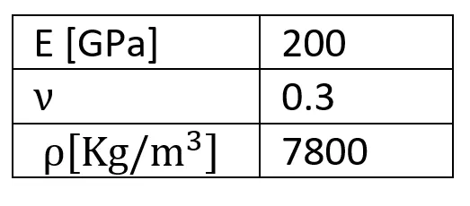
The same material was assigned to both parts. The material is steel with the following properties:
The material for body 1 (red) was assigned using a MAT_RIGID card. Body 2 (in blue) was assigned with a MAT_ELASTIC card.
4. Simulation setup
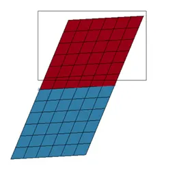
All the nodes contained in the box in the figure below are constrained in all DOF’s.
5. Joint creation
5.1. Revolute joint
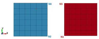
For the definition of the revolute joint, the 4 nodes selected are:
5.2. Spherical joint
The definition of the nodes for the spherical joint was the same as the one for the Revolute joint, although only N1 and N2 were necessary for the joint formulation
5.3. Cylindrical joint
For the cylindrical joint, the node definition is the same as for the revolute joint definition, the joint type was the only change done.
5.4. Translational joint
The node definition for the translational joint was kept the same, with the difference that, this time, two additional nodes were defined to define the orthogonal constraint direction.
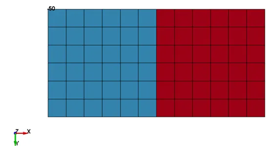
These nodes are contained in rigid bodies. The next image shows the rigid body created on the part 2 side to aid the implementation of the translational joint.
6. Imposed motion
6.1. Revolute joint
To see whether the joints are performing correctly or not, the rigid body will rotate around the axis that separates both.
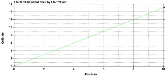
This will be done by imposing on NID = 50 a displacement of 20 mm in the z direction.
The curve defined in LS-Dyna to impose the position of the DOF 3 at this node is the following:
Node ID 50 indication
The type of joint to be created is CONSTRAINED_JOINT_REVOLUTE
6.2. Spherical joint
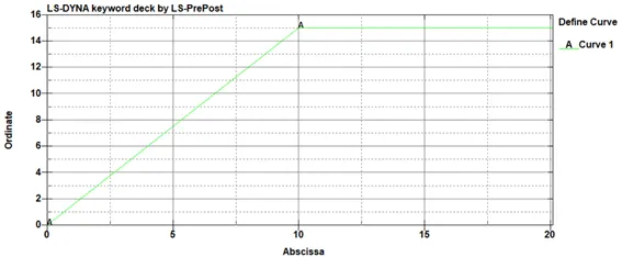
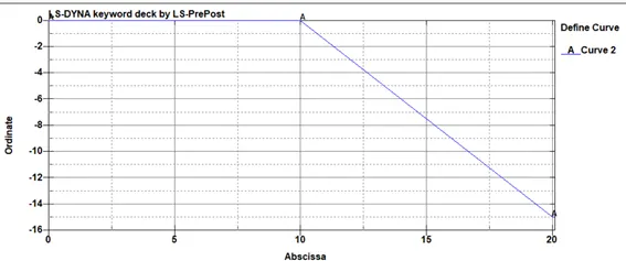
In this case, two movements will be imposed on nodes 50 and 57 to verify the behavior of the joint.
Movement on node 50 (DOF = 3):
6.3. Cylindrical joint
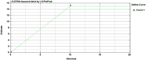
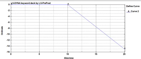
For this joint, the imposed displacement was the following:
Imposed displacement on node 53 (DOF = 3)
Imposed displacement on node 53 (DOF = 2)
6.4. Translational joint
For the translational joint, the same imposed displacement as for the cylindrical joint will be considered.
7. Results
7.1. Revolute joint
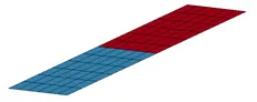
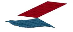
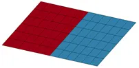
The following figures display the result of the simulation results for each joint type. From these figures and considering the imposed displacements mentioned before, it can be concluded that the joints appear to be behaving accordingly.
7.2. Spherical joint
Initial position Final position
7.3. Cylindrical joint
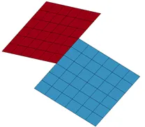
Initial position Final position
7.4. Translational joint
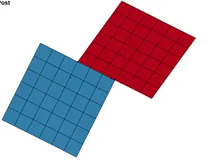
8. Results
As shown in the results' images, the joints appear to be beahving as expected, respecting the constrained DOF's.
For the Translational joint, twi nodes on the blue body were included in a rigid body. This rigidbody is the one who enters the Translational joint formaulation. Therefore, the behaviour of this joint is simillar (if not equal) to the one from the cylindrical joint.