Week-11 : Discretization of 3D intake manifold using GEM-3D

Discretization of 3D intake manifold using GEM-3D

Objectives:

1. Explore Tutorial- single cyl DI with discretization length 0.1 mm for intake runner and compare its computation time with default case.

2. Explore (GEM3D) - “Building intake manifold from STL model”

Numerical Discretization:

Discretization is the process of replacing a continuum with a finite set of points. It is the process to convert a continuous equation into a form that can be used to calculate numerical solutions.

Here, in GEM 3D a 3D model is converted into equivalent 1D GT model in which discretization length can be specified as per user and results can be obtained equivalent to 3D simulation. However, this does not yield very detailed output such as a requirement in simulation of shockwaves. In those cases, 3D simulation yields better results.

Discretization Length:

The smallest length by which the geometry is divided into equal elements. Smaller the Discretization Length, Higher the Accuracy and Computation Time. However, increasing the Discretization Length beyond the limit of Courant Number leads to diverging of solution.

Explicit Method:

In explicit schemes, the information at time n+1 depends on the n. They are computationally fast but stability of the solution depends on Courant Number.

Courant Number:

The Courant number is a dimensionless value representing the time a particle stays in one cell of the mesh. It must be below 1 and should ideally be below 0.7. If the Courant number exceeds 1, the time step is too large to see the particle in one cell, it “skips” the cell. If it is smaller than 0.7, the particle stays in the cell for at least two time steps. The picture below visualizes this situation.

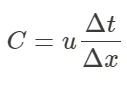
where C is Courant number, u is velocity magnitude, Δt is time step size and Δx is the Discretization length.

1. Exploring the effect of discretization length in the Tutorial "Single Cylinder DI engine" model

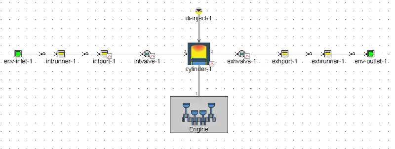
Fig. Single Cylinder DI engine Model

Case Setup:

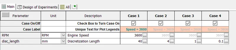
The model is set up with 4 cases, each at 3600 RPM. The discretization length of the inlet manifold is defined as a user defined variable and varied from 40 to 0.1 mm

Results:

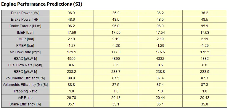
• In the below table, it is evident that almost all the results across four cases vary by a very negligible margin. However this might not be the case for any other simulations. Here, Case 4 with 0.1 mm of discretization length should be the most accurate result among others.

• The below table shows that the case has been solved using explicit technique. Number of flow volumes represents number of elements the runner is discretized into. It can be observed that both elements and timesteps increases when discretization length decreases.

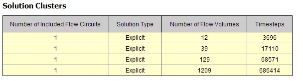
• Main objective of this study is to investigate the effect of discretization length in computation time. The below table shows that the time taken increases as discretization length decreases. Decreasing the discretization length leads to better accurate results provided it is in acceptable courant number in case of explicit solutions.

2. Discretization of intake manifold (3D model to 1D using GEM3D)

Step 1: The imported 3D intake manifold has been fluid volume extracted and exported as a STL file (Standard Triangle Language) using GT-Spaceclaim tool.

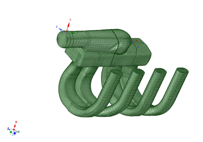
Step 2: STL geometry is imported into GEM 3D

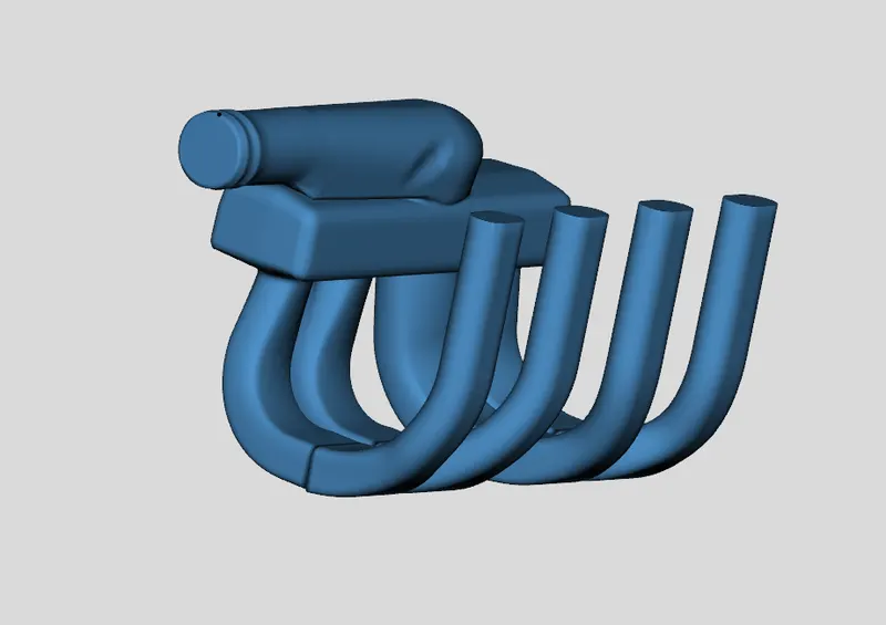
Step 3: Now, the main objective is to convert the 3D model into equivalent 1D model. The inlet and outlet surfaces are removed so as to simply them as different equivalent parts. The geometry is further "separated by curves" which makes the four outlets as different structure as highlighted.

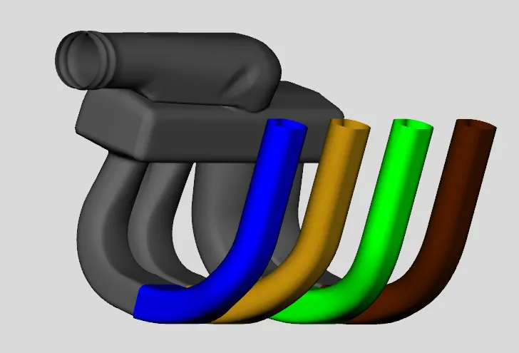
Step 4: The remaining part of the outlets are separated from the separation chamber using 3 point cutting plane at the plenum (marked as red).

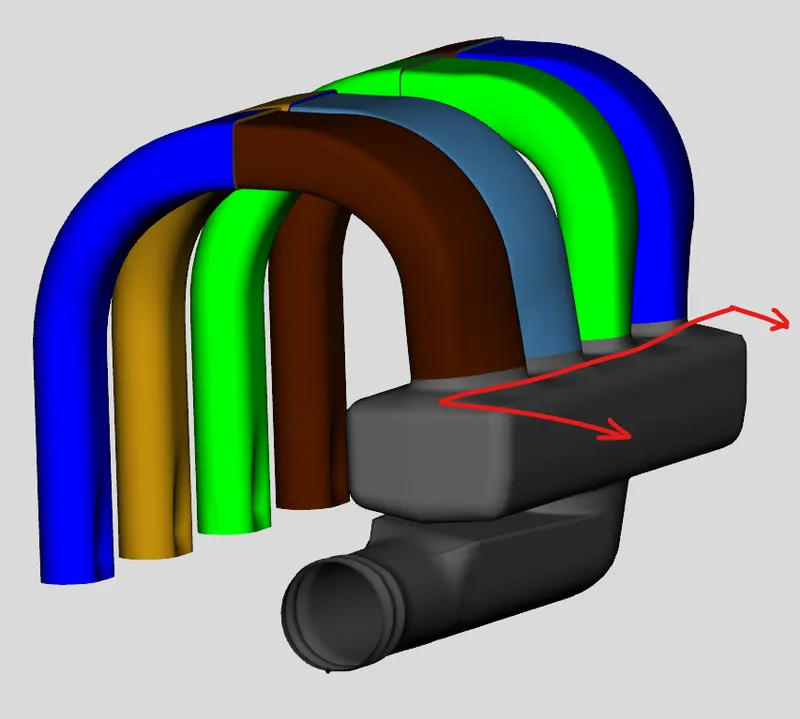
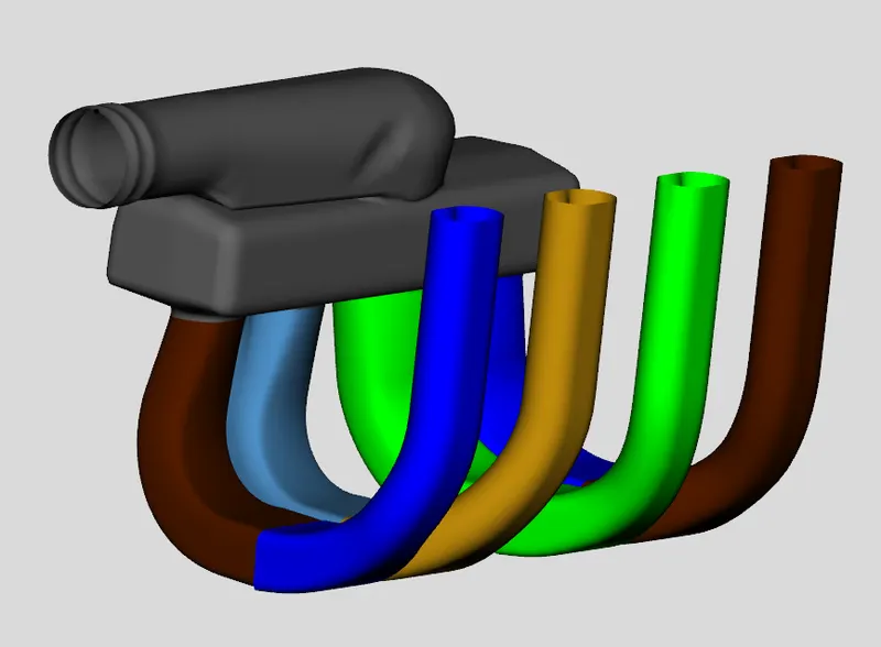
Step 5: If above images are observed, it is very much clear that the shapes of outlets are not exactly circular. In order to simplify the model, the direction of flow is assigned to the outlets (Fig. A) relevent dimensions and properties are added (Fig.B and C). All are converted into pipes with multiple bends.

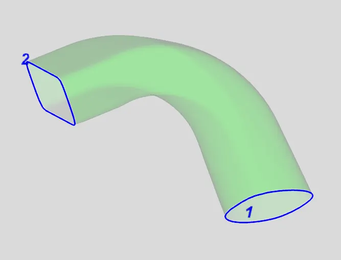
Fig A. Flow direction

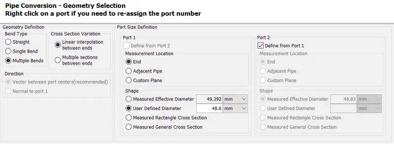
Fig B . Conversion of uneven shape to known shape

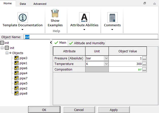
Fig C. Properties assigned to all 8 outlet ports

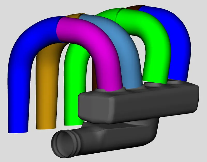
Fig D. Outlets ports with circular cross section

Step 6: Now inlet ports are divided into two sections using section plane and all ports are assigned with orifice connection and extension connection (ExtConn)

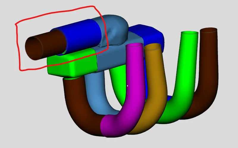
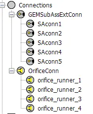
Step 7: Here the manifold is divided into 3 regions and flow split applied.

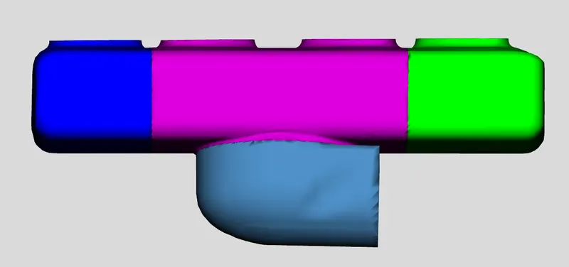
Step 8: At last the entire geometry is given a flow connection at the gaps so as to make them as continuous flow domain and the geometry is exported as a GT model.

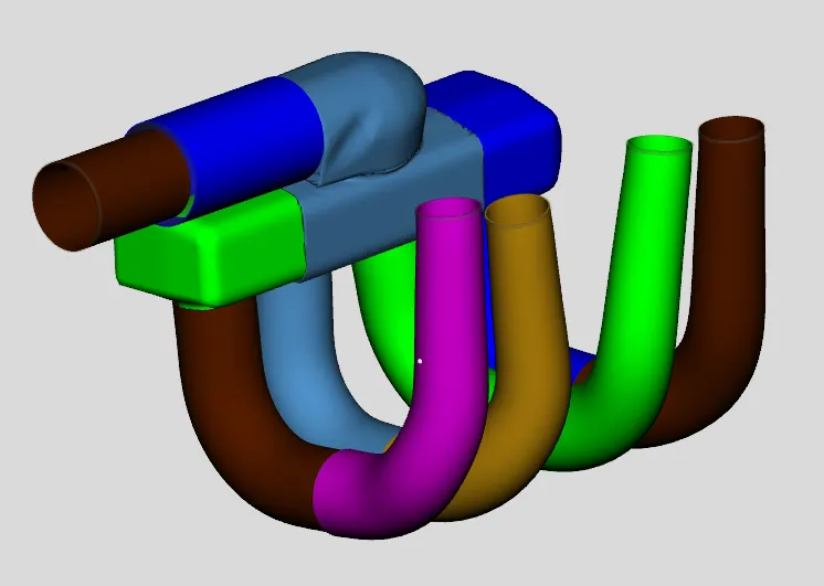
Result: (3D model to 1D GT model)

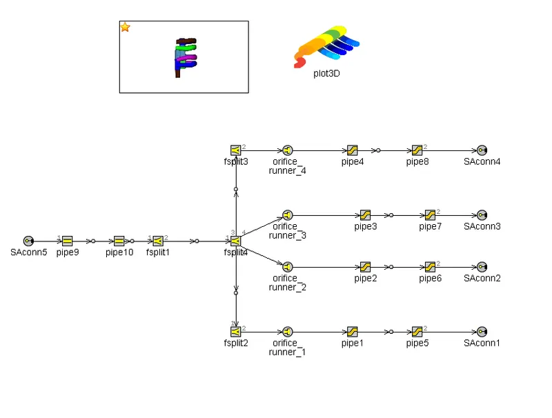
Fig. 1D model of 3D intake manifold

• SAconn1,2,3,4 represents the outlet end of the manifold and SAconn5 represents the inlet.
• pipe9 and 10 represents the inlet end of intake manifold.
• fsplit1 represents the bend pipe towards plenum.
• plenum is splitted further into 3 splits (fsplit 2,3,4)
• fsplits are further divided into orifice_runner_1,2,3,4 which is joined further by the outlet ends (pipe 1,2,3,4,5,6,7,8)
• SAconn1,2,3,4 are the outlets which can be connected to any of the engine model.

References:

[1] https://www.simscale.com/knowledge-base/what-is-a-courant-number/