Week-11 Challenge: Braking

1.

    Braking:

     Braking is a condition to slow down or stops a moving vehicle as required. There are several techniques to apply brakes, which can be mechanical or electrical. The most commonly used technique is by applying friction. It consumes energy.

        Braking Energy = (1/2)*m*v^2

            where,m= Total Mass of the Vehicle in kg

                      v=velocity (initial velocity-final velocity) m/s

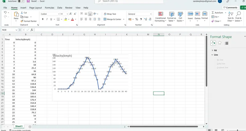
Here for a Drive cycle the required braking energy is calculated for each second of time to slow down or stop the vehicle;

2.

There are two types of braking:

1.Mechanical Braking:

 Mechanical brakes all act by generating frictional forces as two surfaces rub against each other. The stopping power or capacity of a brake depends largely on the surface area of frictional surfaces as well as on the actuation force applied. Mechanical brakes are assemblies consisting of mechanical elements for the slowing or stopping of shafts in equipment drives. They use levers or linkages to transmit force from one point to another. Braking slows or stops the movement of the coupled shafts. There are several types of mechanical brakes.

i) Band brakes: These are the simplest brake configuration, have a metal band lined with heat and wear resistant friction material.

ii)Drum brakes: These are commonly used on automobile rear wheels, work when shoes press against a spinning surface called a drum.

iii)Disc brakes: These are constructed of brake pads, a calliper, and a rotor. During operation, the brake pads are squeezed against the rotor.

2. Electrical Braking: 

Electric brakes are devices that use an electrical current or magnetic actuating force to slow or stop the motion of a rotating component. They are used in industrial and vehicular braking applications that require fast response times and precise tension control. The magnet in the backing plate has 2 conductor wires which tap directly into the wiring. When electricity is on, it magnetizes the brake magnet. The magnet is attracted to the drum face. When it contacts this area, the friction causes it to rotate, which moves the actuating arm, and pushes the shoes out against the drum. Those shoe have a special brake pad material on them that resists the heat caused by that friction. When the shoes press against the inside of the drum, they prevent the hub, and consequently the wheel that's touching the ground.

A very beautiful electric braking scheme called Regenerative Braking is now being employed for electric braking. Here during the braking action, the motor is operated as generator. As we know that during generating action, a counter torque is produced. So this counter torque opposes the motion of motor and motor comes to halt. Moreover, the brake energy is converted to electrical energy which can be fed back to the source using power converters.

Electric and Mechanical brake coordination:

There are mainly 2 ways by which the Electric Vehicles could be braked:

• Series- Regenerative braking and mechanical braking both are applied one after another.
• Parallel- Regenerative braking and mechanical braking both are applied simultaneously.

      When brake pedal is pressed the hydraulic fluid reaches the brake pistons and created the braking pressure on the wheels and the same kinetic energy is been used by the Regenerative Braking for generating more power using the Bi-directional motor which operates as a generator while braking.

3.

Matlab program:

clear all
close all
clc

% Speed
omega = linspace(0, 300, 100);

% Torque 
T = linspace(0, 2000, 100);

% Meshgrid
[X,Y] = meshgrid(T, omega);

% Loss Coefficients
% Copper coefficient
cu = 0.17;   
% Iron coefficient
fe = 0.006;    
% Windage coefficient
win = 0.000015;          

% Losses
% Copper Losses
cu_loss = cu*(Y.^2);
 % Iron Losses
fe_loss = fe*(X.^2); 
 % Windage Losses
win_loss = win*(X.^3);
% Conduction Losses
cond_loss = 18; 

% Output Power
P_out = (X.*Y);

% Input Power
P_in = P_out + (cu_loss) + (fe_loss) + (win_loss) + (cond_loss);

% Efficiency
n = ((P_out)./(P_in));

% Efficiency values for contour
W = linspace(0.75, 0.95, 10);

% Contour Plot
contour(X,Y,n,W)
xlabel('Angular Speed (rad/s)')
ylabel('Torque (Nm)')
title('Speed, Torque and Efficiency characteristics of Motor')

Result:

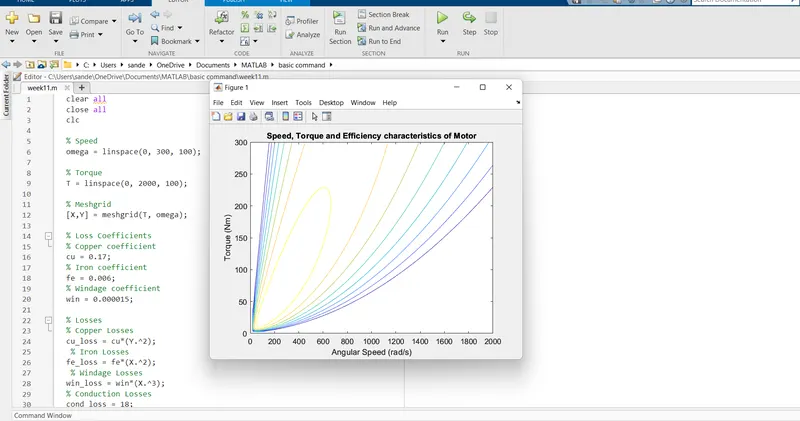
From this contour plot, we can see that the highest level of efficiency arises in the innermost contour plot and this efficiency decreases as the contours increase in size from the innermost contour.