Week-11 Challenge: Braking
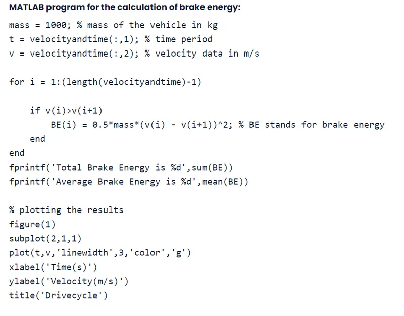
Q.1 For a defined driving cycle, calculate the energy required for braking.
Solution:-
Eectric motor can't develop braking torque at high speed similar to starting, because Braking torque is applied in the opposite direction of the rotation. We can use a mechanical brake to produce a braking torque.
Abstract
The market segment of hybrid-electric and full function electric vehicles is growing within
the automotive transportation sector. While many papers exist concerning fuel economy or fuel
consumption and the limitations of conventional powertrains, little published work is available
for vehicles which use grid electricity as an energy source for propulsion. Generally, the
emphasis is put solely on the average drive cycle efficiency for the vehicle with very little
thought given to propelling and braking powertrain losses for individual components. The
modeling section of this paper will take basic energy loss equations for vehicle speed and
acceleration, along with component efficiency information to predict the grid energy
consumption in AC Wh/km for a given drive cycle.
This paper explains how to calculate the forces experienced by a vehicle while completing a
drive cycle in three different ways: using vehicle characteristics, United States Environmental
Protection Agency‟s (EPA) Dynamometer „target‟ coefficients, and an adaptation of the Sovran
parameters. Once the vehicle forces are determined, power and energy demands at the wheels
are determined. The vehicle power demands are split into propelling, braking, and idle to aide in
the understanding of what it takes to move a vehicle and to identify possible areas for
improvement. Then, using component efficiency data for various parameters of interest, the
energy consumption of the vehicle as a pure EV is supplied in both DC (at the battery terminals)
and AC (from the electric grid) Wh/km. The energy that flows into and out of each component
while the vehicle is driving along with the losses at each step along the way of the energy path
are detailed and explained. The final goal is to make the results of the model match the vehicle
for any driving schedule. Validation work is performed in order to take the model estimates for
efficiencies and correlate them against real world data. By using the Virginia Tech Range
Extended Crossover (VTREX) and collecting data from testing, the parameters that the model is
based on will be correlated with real world test data. The paper presents a propelling, braking,
and net energy weighted drive cycle averaged efficiency that can be used to calculate the losses
for a given cycle. In understanding the losses at each component, not just the individual
efficiency, areas for future vehicle improvement can be identified to reduce petroleum energy
use and greenhouse gases. The electric range of the vehicle factors heavily into the Utility
Weighted fuel economy of a plug-in hybrid electric vehicle, which will also be addressed.
The market segment of hybrid-electric and full function electric vehicles is growing within
the automotive transportation sector. While many papers exist concerning fuel economy or fuel
consumption and the limitations of conventional powertrains, little published work is available
for vehicles which use grid electricity as an energy source for propulsion. Generally, the
emphasis is put solely on the average drive cycle efficiency for the vehicle with very little
thought given to propelling and braking powertrain losses for individual components. The
modeling section of this paper will take basic energy loss equations for vehicle speed and
acceleration, along with component efficiency information to predict the grid energy
consumption in AC Wh/km for a given drive cycle.
This paper explains how to calculate the forces experienced by a vehicle while completing a
drive cycle in three different ways: using vehicle characteristics, United States Environmental
Protection Agency‟s (EPA) Dynamometer „target‟ coefficients, and an adaptation of the Sovran
parameters. Once the vehicle forces are determined, power and energy demands at the wheels
are determined. The vehicle power demands are split into propelling, braking, and idle to aide in
the understanding of what it takes to move a vehicle and to identify possible areas for
improvement. Then, using component efficiency data for various parameters of interest, the
energy consumption of the vehicle as a pure EV is supplied in both DC (at the battery terminals)
and AC (from the electric grid) Wh/km. The energy that flows into and out of each component
while the vehicle is driving along with the losses at each step along the way of the energy path
are detailed and explained. The final goal is to make the results of the model match the vehicle
for any driving schedule. Validation work is performed in order to take the model estimates for
efficiencies and correlate them against real world data. By using the Virginia Tech Range
Extended Crossover (VTREX) and collecting data from testing, the parameters that the model is
based on will be correlated with real world test data. The paper presents a propelling, braking,
and net energy weighted drive cycle averaged efficiency that can be used to calculate the losses
for a given cycle. In understanding the losses at each component, not just the individual
efficiency, areas for future vehicle improvement can be identified to reduce petroleum energy
use and greenhouse gases. The electric range of the vehicle factors heavily into the Utility
Weighted fuel economy of a plug-in hybrid electric vehicle, which will also be addressed.
Q.2Why electric motor can’t develop braking torque at high speed similar to starting? How electric and mechanical brakes are coordinated
solution:-
Eectric motor can't develop braking torque at high speed similar to starting, because Braking torque is applied in the opposite direction of the rotation. We can use a mechanical brake to produce a braking torque
HEV Structure and Dynamic Model
2.1. HEV Structure
The structure of a plug-in hybrid vehicle, as shown in Figure 1, mainly includes an engine, an ISG motor, a permanent magnet synchronous motor (PMSM), a dual clutch, and an infinitely variable transmission (CVT). The front axle is driven by the engine and the integrated starter generator (ISG), the rear axle is driven by the PMSM, and the dual clutch is mounted on both ends of the ISG motor.
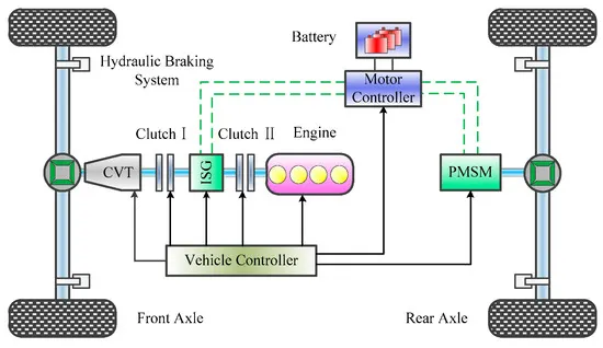
Figure 1. Structure of a plug-in hybrid vehicle.
2.2. Dynamic Model
2.2.1. Motor Dynamic Model
The three-phase PMSM is a strongly coupled and multivariable nonlinear system [13]. In order to accurately reflect the dynamic response characteristics of the motor during braking, a dynamic model is established based on the mathematical model of the three-phase PMSM. In the synchronous rotating coordinate system (d-q axis), the ideal PMSM voltage equation [14] is:
{ud=Rid+Ldddtid−ωeLqiquq=Riq+Lqddtiq+ωe(Ldid+ψf)
The electromagnetic torque equation is:
where ud, uq respectively represent the stator voltage d-q axis component; id, iq respectively represent the stator current d-q axis component; R is stator resistance; ωe is electrical angular velocity; Ld, Lq respectively represent inductance d-q axis component; ψf is permanent magnet flux chain; pn is motor pole pairs.
Te=32pniq[id(Ld−Lq)+ψf]
2.2.2. Hydraulic Dynamic Model
The dynamic response characteristics of the hydraulic braking system are related to the hydraulic system structural parameters, duty cycle and so on. However, building a precise model of the hydraulic braking system is difficult and the required computational power is large. In order to simplify the model and accurately reflect the dynamic characteristics of the hydraulic system, this study uses the empirical first-order inertia link [15]:
where Thf, Thr are the front and rear axle brake torque; Pf, Pr are cylinder pressures; Df, Dr are axle cylinder diameter; Rf, Rr are brake operating radius; BFf, BFr are brake efficiency factors; τ is the first-order system time constant, which can be obtained by experience; s is a variable.
{Thf=Pf14πD2fRfBFf1sτ+1Thr=Pr14πD2rRrBFr1sτ+1
As shown in Figure 2, the motor torque response is quick and accurate, the response time is approximately 0.06 s, and the overshoot is 11.12%. Compared with the motor, in order to overcome the brake clearance and cylinder pressurization, the hydraulic system’s torque response is slow but stable and the response time is approximately 0.17 s. According to [16], the full starting time of the driving brake is generally controlled within 0.2–0.3 s; thus, the dynamic response characteristics of the hydraulic model constructed in this study satisfies this requirement.
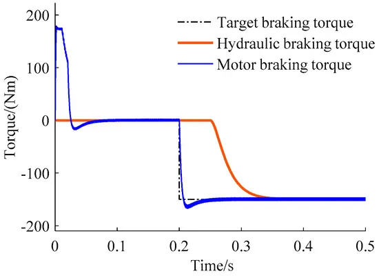
Figure 2. Step response of motor and hydraulic braking torque.
2.2.3. Engine Drag Model
When the engine is anti-dragged, the throttle is closed and the engine drag resistant torque is related to the engine speed, as shown in Figure 3. Because the engine has multiple subsystem modules, the establishment of the engine model is difficult. At the same time, this study does not consider the problem of engine emissions. Therefore, this study uses the experimental modeling method to establish the engine model, and the output response of the engine drag resistant torque is characterized by a second-order transfer function:
where ωn is the natural frequency; ζ is the damping coefficient; ne is the engine speed; TbICE is the engine drag resistant torque; s is a variable.
TbICE=ω2ns2+2ζωns+ω2nf(ne)
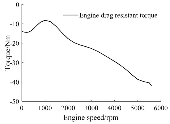
Figure 3. Engine drag resistance torque.
3. Braking Force Distribution Strategy
The hybrid electric vehicle mentioned above is equipped with dual motors, and during braking, the maximum strength of the motor brake ranges from 0.06 to 0.27 with the speed and CVT ratio changing. Therefore, in order to recover as much energy as possible, this study puts forward a brake force distribution strategy based on the motor braking capacity, while taking the engine brake into consideration.
The braking force distribution curve is shown in Figure 4. V is the speed of the vehicle; Vmax and Vmin are the maximum and minimum vehicle speeds allowed for regenerative braking; SOChigh is the maximum state of charge allowed for regenerative braking; io1 and io2 are the transmission ratios of final drive I and final drive II; icvt is the CVT transmission ratio; z is the braking strength; Fb_req is the total braking force the driver demanded; Fbm_req, Fbh_req and FbICE_req are the target motor, hydraulic and engine braking forces; Fbxf_req and Fbxr_req are the target braking forces of the front and rear axles of the vehicle; Fbhf_req and Fbhr_req are the target hydraulic braking forces of the front and rear axles; FbI_req and FbP_req are the target braking forces of ISG and PMSM; FbI_max and FbP_max are the maximum braking forces that ISG and PMSM can provide in the current state; FbICE is the engine drag resistant force; Fbm_max is the maximum braking force that the motor can provide; β is the ratio between front axle and total braking force.
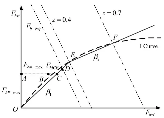
Figure 4. The braking force distribution curve. (Fbxf) Braking force in the front axle; (Fbxr) braking force in the rear axle; (I curve) the ideal braking force distribution curve.
As seen in Figure 4, the point E is the intersection of line z = 0.4 and curve I while the point F is the intersection of line z = 0.7 and curve I. Therefore, the β line consists of the OE and EF segments and the braking strengths of A, B and C are:
⎧⎩⎨⎪⎪⎪⎪⎪⎪⎪⎪z(A)=io2FbP_maxGz(B)=Fbm_maxGz(C)=io2FbP_max(1+β1)G
The required motor braking force is:
Fbm_req=icvtio1FbI_req+io2FbP_req
The required hydraulic braking force is:
Fbh_req=Fbhf_req+Fbhr_req
The required braking force is:
Fb_req=Gz
The detailed braking force distribution strategies are as follows:
When Vmin < V < Vmax and SOC < SOChigh:
(1) 0 < z ≤ z(B)
In this condition, braking force is completely provided by the regenerative braking force. Fbh_req = 0, Fbm_req = Fb_req. The braking forces of ISG and PMSM are distributed as follows:
When 0 < z ≤ z(A),
{FbI_req=0FbP_req=Fb_reqio2
When z(A) < z ≤ z(B),
{FbI_req=Fb_req−io2FbP_maxicvtio1FbP_req=FbP_max
(2) z(B) < z ≤ z(C)
In order to make full use of engine to brake, the braking force is provided by the motor and the engine braking system. Therefore, Fbh_req = 0, Fb_req = Fbm_req + icvtio1FbICE.
⎧⎩⎨⎪⎪⎪⎪⎪⎪FbICE_req=FbICEFbI_req=Fb_req−io2FbP_maxicvtio1−FbICEFbP_req=FbP_max
(3) z(C) < z ≤ z(F)
When z(C) < z ≤ z(F), the braking force is provided by the motor and the hydraulic braking system. The target braking forces of the front and rear axles, distributed in accordance with line CEF shown in Figure 4, are Fbxf_req and Fbxr_req. Therefore, FbICE = 0, Fb_req = Fbm_req + Fbh_req. The braking forces of the motor and hydraulic braking system are:
⎧⎩⎨⎪⎪⎪⎪⎪⎪⎪⎪FbI_req=FbI_maxFbP_req=FbP_maxFbhf_req=Fbxf_req−icvtio1FbI_maxFbhr_req=Fbxr_req−io2FbP_max
When V > Vmax or V < Vmin or SOC ≥ SOChigh or z > z(F), the braking force is completely provided by the hydraulic braking system. The braking forces of the hydraulic braking system are:
{Fbhf_req=Fbxf_reqFbhr_req=Fbxr_req
4. Coordinated Control Strategy for Braking Mode Switch
4.1. Kinetics Analysis of Braking Mode
According to the braking force distribution control strategy mentioned above, there are four main braking modes: pure electric braking mode, motor and engine braking mode, motor and hydraulic braking mode, and hydraulic braking mode. In order to facilitate the kinetic analysis, the hybrid vehicle drive system model is simplified, as illustrated in Figure 5. where Je is moment of inertia of the engine; JISG is moment of inertia of the ISG; Jcvt is moment of inertia of the CVT; JC1 is moment of inertia of the clutch I; JC2 is moment of inertia of the clutch II; JPMSM is moment of inertia of the PMSM; Jw is moment of inertia of the wheel; JO1 is moment of inertia of the final drive I; JO2 is moment of inertia of the final drive II; m is the vehicle mass; r is the tire radius.
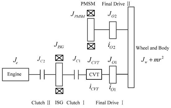
Figure 5. Equivalent diagram of the system model.
(1) Pure Electric Braking Mode
When the motor is braking clutch I is engaged and clutch II is disconnected. The engine and the hydraulic braking systems do not participate in the braking action and the required braking torque is provided by the motor. The equivalent to the moment of inertia on the wheel is:
Jv=((JISG+JC1)⋅icvt+JCVT)⋅iO1+JO1+JO2+JPMSM⋅iO2+Jw+mr2
The dynamic equation of braking is:
where TbICE is the engine drag resistance torque, Tbh is the hydraulic braking torque, TbISG is the ISG braking torque, TbPMSM is the PMSM braking torque, and ω˙w is the wheel angular acceleration.
⎧⎩⎨⎪⎪TbICE=0Tbh=0TbISG⋅icvt⋅iO1+TbPMSM⋅iO2=Jvωw∙
(2) Motor and Engine Braking Mode
When the motor and engine are involved in braking, clutches I and II are engaged. The required braking torque is provided by the motor and the engine. At this time, the equivalent to the moment of inertia on the wheel is:
Jv=((Je+JISG+JC1+JC2)⋅icvt+JCVT)⋅iO1+JO1+JO2+JPMSM⋅iO2+Jw+mr2
The dynamic equation of braking is:
{Tbh=0(TbISG+TbICE)⋅icvt⋅iO1+TbPMSM⋅iO2=Jvωw∙
(3) Motor and Hydraulic Braking Mode
During motor and hydraulic braking modes, clutch I is engaged and clutch II is disconnected. The required braking torque is provided by the motor and the hydraulic braking system. At this time, the equivalent to the moment of inertia on the wheel is:
Jv=((JISG+JC2)⋅icvt+JCVT)⋅iO1+JO1+JO2+JPMSM⋅iO2+Jw+mr2
The dynamic equation of braking is:
{TbICE=0TbISG⋅icvt⋅iO1+TbPMSM⋅iO2+Tbh=Jvωw∙
(4) Hydraulic Braking Mode
During hydraulic braking mode, clutches I and II are disengaged and the required braking torque is provided by the hydraulic braking system. The equivalent to the moment of inertia on the wheel is:
Jv=JCVT⋅iO1+JO1+JO2+JPMSM⋅iO2+Jw+mr2
The dynamic equation of braking is:
⎧⎩⎨⎪⎪TbICE=0TbISG=TbPMSM=0Tbh=Jvωw∙
Based on the kinetics analysis of the braking mode, there are three types of braking torque that need to be coordinated during braking mode switching. The motor, the hydraulic, and the engine braking systems are three different systems with different dynamic response characteristics; therefore, the sequences and moments of the three joint systems are different. Because mode switching is completed instantaneously, the braking torque varies sharply during the intervention and exit from braking. If there is no coordinated control, it will cause torque fluctuation and seriously worsen the ride comfort of the vehicle.
4.2. Coordination Control Strategy for Mode Switch
According to whether or not the hydraulic braking system is involved in braking, the braking mode-switch type is divided into two categories (Figure 6). Braking mode-switch coordination control strategies are developed for the different braking mode-switch types.
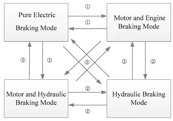
Figure 6. Braking mode switch classification.
(1) Type one: braking mode switch without hydraulic braking system participation. In this type of mode switching it is necessary to control the engagement of the clutch and the change rate of the motor torque. Thus, the fluctuation caused by mode switch can be reduced.
(2) Type two: braking mode switch with hydraulic braking system participation. Due to the different dynamic response characteristics of the motor and the hydraulic braking systems, this switch mode is difficult to coordinate. The idea of coordinating control is to take full advantage of the characteristics of the braking systems. The hydraulic system can provide large and stable torque, and the motor braking system’s torque response is quick and accurate, reducing the fluctuation of the vehicle.
The overall coordination control flow chart is shown in Figure 7. Tbm_req, Tbh_req and TbICE_req are the target motor, hydraulic and engine braking torques allocated by the braking force control strategy.
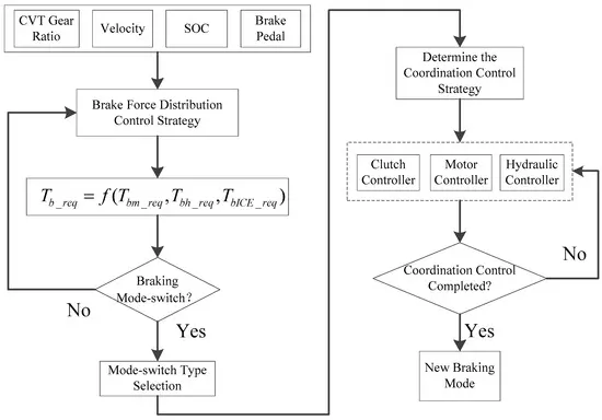
Figure 7. Flow chart of overall coordination control.
First, according to current speed, SOC, CVT ratio, and brake pedal, the braking force distribution control strategy allocates the target motor, hydraulic and engine braking torques; then, according to the braking mode boundary conditions the vehicle controller determines whether the braking mode should switch or not. If mode switching happens, the vehicle controller determines the type of mode switch and then selects the corresponding coordination control strategy and controls the clutch, motor and hydraulic torques to reduce the mode switch fluctuation. Finally, the vehicle controller determines whether the coordination control is completed, and if it is completed, the vehicle will enter a new braking mode.
4.2.1. Coordination Control Strategy of Type One
In this type of mode switch the motor braking torque and the engine drag resistance torque, transmitted by clutch II, are the main sources of braking torque fluctuation. Therefore, the braking torque fluctuation is coordinated by controlling the change rate of the clutch hold-down force and the motor brake force. The torque transmitted by the dry clutch during slipping is:
where Δω is the clutch angular velocity difference between the main and driven plate; sign is symbolic function; μ is clutch friction factor, which is related to the surface temperature of the plates and Δω; F(t) is the compression force of clutch plates; Z is the clutch friction pair number; R0, R1 are the clutch outer and inner friction plate diameter.
Tc=sign(Δω)23μF(t)ZR30−R31R20−R21
The coordinated control flow chart of type one is shown in Figure 8, km and kc are the change rates of motor brake torque and clutch hold-down force. Tbm and Tc are the actual torques of motor and clutch and Tbm = TbISGicvtio1 + TbPMSMio2. Tb is the actual total brake torque.
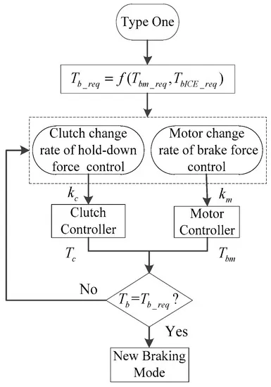
Figure 8. Flow control chart of the first type mode-switch.
It is simple to control the motor brake force changing rate, however, it is hard to obtain the target change rate of the clutch hold-down force. Moreover, it is assumed that the target change rate of the total brake force is kreq. Thus:
where F0, Tbm0 and Tb0 are the initial values of the clutch hold-down force, the motor brake torque, and the total brake force.
⎧⎩⎨⎪⎪⎪⎪⎪⎪⎪⎪⎪⎪⎪⎪⎪⎪⎪⎪F(t)=F0+∫kcdtTbm(t)=Tbm0+∫kmdtTb(t)=Tb0+∫kreqdt
Then:
Tb(t)=Tbm(t)+Tcicvtio1
Derivation of the formula above gives:
and:
kreq=km+aicvtio1kc
a=sign(Δω)μZR
Therefore, the change rate of clutch hold-down force is:
kc=kreq−kmaicvtio1
4.2.2. Coordination Control Strategy of Type Two
The dynamic response of the hydraulic braking system is slow and stable while the response of the motor braking system is fast and accurate. The hydraulic brake system has been developed for a long time, its technology is mature and stable, and its dynamic response characteristics have been well researched [17]. Therefore, in order to make full use of the characteristics of the motor and the hydraulic braking systems, the coordinated control process of braking mode switch is divided into two stages; this is achieved by modifying the target braking torque.
The coordinated control flow chart of type two is shown in Figure 9, Tbm′, Tbh′ and TbICE′ are the modified target braking torques of the motor, the hydraulic and the engine braking system; Tbm0, Tbh0 and TbICE0 are the initial torques of the motor, the hydraulic and the engine braking system when mode is switched; Tc is the transmitted torque of the dry clutch. When mode switch happens, the coordination control process is described as follows: during mode switching, the torques of the motor, the hydraulic and the engine braking system are:
⎧⎩⎨⎪⎪Tbm=Tbm0Tbh=Tbh0TbICE=TbICE0
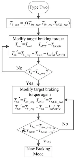
Figure 9. Flow control chart of the second type mode-switch.
At that moment, the coordinated control process of the braking mode switch enters into the first stage: it keeps the brake torques of the motor and engine unchanged and modifies the target braking torque of the hydraulic braking system to meet the driver demand. Therefore, the modified torques are:
⎧⎩⎨⎪⎪Tbm′=Tbm0Tbh′=Tb_req−Tbm0−icvtio1TbICE0TbICE′=TbICE0
Next, the vehicle controller determines whether Tb is equal to Tb_req, if Tb = Tb_req, the coordinated control process enters into the second stage: it makes full use of the dynamic characteristics of the motor braking system to coordinate the torque fluctuation and modifies the target braking torque of the engine and the hydraulic braking system in order to reach the target value (Tbh_req and TbICE_req)
⎧⎩⎨⎪⎪Tbm′=Tb_req−Tbh−icvtio1TcTbh′=Tbh_reqTbICE′=TbICE_req
Finally, the vehicle controller evaluates whether Tbm = Tbm_req and TbICE = TbICE_req if so, the current mode is substituted by a new braking mode.
A motor torque proportional-integral-derivative (PID) control algorithm was designed in order to improve the hydraulic and clutch torque fluctuation and keep the total braking torque stable during the second stage. The PID algorithm’s control structure is shown in Figure 10. The input is Tbm′ which is the modified target braking torque of the motor while the output is Tbm which is the actual braking torque of the motor.
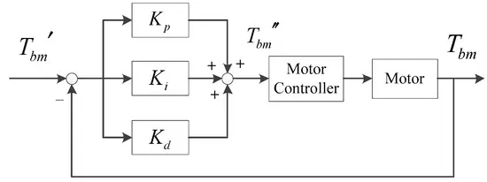
Figure 10. Motor torque PID control algorithm.
The PID control algorithm’s expression is:
where e(t) is the PID deviation; Kp, Ki and Kd are the PID ratio, the integral and the differential factors.
⎧⎩⎨⎪⎪Tbm′′=Kpe(t)+Ki∫e(t)dt+Kdddte(t)e(t)=Tbm′−Tbm
5. Simulation Results and Analysis
In this study, the simulation model of a plug-in four-wheel drive hybrid vehicle was established on the MATLAB/Simulink simulation platform. The parameters of the hybrid vehicle and the key components are listed in Table 1. The effectiveness of the coordinated control strategy was studied by comparing the results with and without a control strategy. In the simulation of the non-coordinated control strategy, motor, hydraulic and clutch torques are not intervened during the braking mode switch while the other parameters remained the same.
Table 1. The parameters of vehicle and key components.

In this paper, the forward simulation model of plug-in hybrid vehicle is established based on MATLAB/Simulink, as illustrated in Figure 11. The vehicle simulation model is composed of ISG model, PMSM model, battery model, hydraulic braking system model and the controller model.
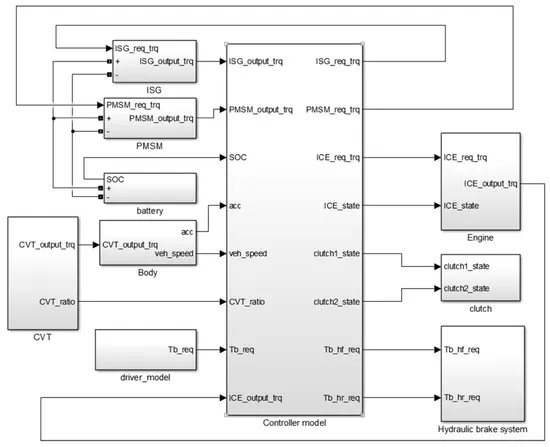
Figure 11. Vehicle simulation model based on Simulink.
The hybrid vehicle’s brake mode-switch types in this study are complex and numerous and it would require a lot of computational power for the simulation analysis of each brake mode switch. Therefore, this study simulated several typical braking mode-switch conditions to verify the effectiveness of the coordinated control strategy. The typical braking mode-switch conditions were as follows: (1) motor braking mode to motor and engine braking mode; (2) motor braking mode to motor and hydraulic braking mode; (3) motor and engine braking mode to motor and hydraulic braking mode; (4) motor and hydraulic braking mode to hydraulic braking mode. This paper takes the urgent situation into consideration, therefore, the step type of target braking force is set, and the simulation results were as follows: when the vehicle speed was 60 km/h and the braking strength was changed from 0.05 to 0.2, the braking mode was switched, at 0.2 s, from the motor brake to the motor and engine brake (Figure 12). In the model without coordination the motor quickly reached the target braking torque due to its rapid response characteristics. The dramatic change of the motor torque had a great impact on the ride comfort of the vehicle, the vehicle jerk caused by the motor reached 86.06 m/s3. Because the clutch was engaged in a slower time than the motor response, it took longer time for it to reach the target value. In the model with coordination, due to fact that the change rate of the motor was limited, the impact caused by the motor torque was significantly improved and the value of vehicle jerk was less than 15.18 m/s3. Therefore, the coordinated control strategy significantly improved the vehicle’s ride comfort.
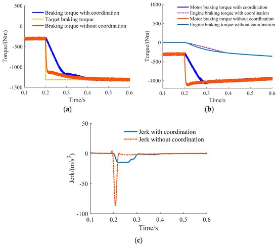
Figure 12. Simulation results of motor braking mode to motor and engine braking mode. (a) Total braking torque; (b) Motor and engine braking torque; (c) Vehicle jerk.
As shown in Figure 13, when the braking strength is changed from 0.1 to 0.3, the braking mode is switched from the motor brake to the motor and hydraulic brake. In the results without coordination the hydraulic system response was slower and the hydraulic braking system reached the target braking torque after the motor, therefore, it had a large impact on the vehicle. In the results with coordination the vehicle fluctuation was significantly improved by coordinating the motor and the hydraulic braking torque. However, a small fluctuation occurred at 0.42 s because the motor did not have enough ability to coordinate the change of the hydraulic braking torque. The jerk of a small fluctuation was less than 1.57 m/s3 and the effect of the coordinated control is pretty good.
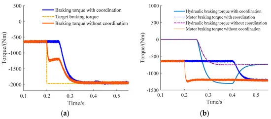
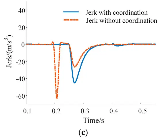
Figure 13. Simulation results of motor braking mode to motor and hydraulic braking mode. (a) Total braking torque; (b) Motor and hydraulic braking torque; (c) Vehicle jerk.
Figure 14 shows that the braking mode changes from motor and engine brake to motor and hydraulic brake. During mode switch, the engine exits the anti-drag brake, and the hydraulic system is involved in braking. Figure 14a shows that the total braking torque fluctuation without coordination is very intense. Meanwhile, the torque fluctuation with coordination is smaller.
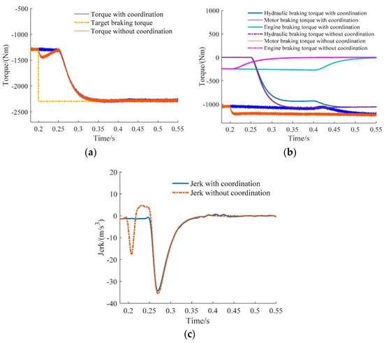
Figure 14. Simulation results of motor and engine braking mode to motor and hydraulic braking mode. (a) Total braking torque; (b) Motor, engine and hydraulic braking torque; (c) Vehicle jerk.
When the mode is switched from motor and hydraulic brake to hydraulic brake (Figure 15), the motor exits the regenerative brake mode, the motor braking torque drops suddenly and the hydraulic braking torque rises slowly. The vehicle jerk without coordination can reach 138.4 m/s3 and the ride comfort is seriously worsened. However, the jerk with coordination is less than 95 m/s3.
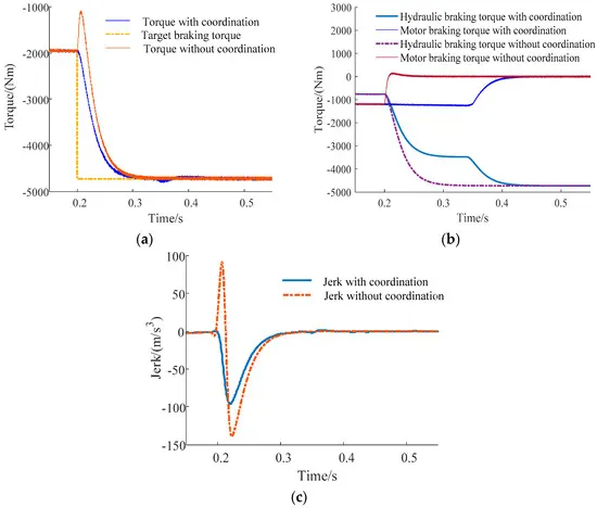
Figure 15. Simulation results of motor and hydraulic braking mode to hydraulic braking mode. (a) Total braking torque; (b) Motor and hydraulic braking torque; (c) Vehicle jerk.
6. Conclusions
In this study, a new type of plug-in hybrid was taken as the research object and the braking force distribution strategy which takes the engine drag resistance torque into consideration was put forward. The types of braking mode switches were divided into two types, aimed at the problem of torque fluctuation during the braking mode switch. Two coordinated control strategies which correspond to the two types were developed by analyzing the clutch and the characteristics of the hydraulic and the motor braking systems. The coordination control strategy of type one was achieved by controlling the change rates of the clutch hold-down force and the motor braking force. By comparing the characteristics of the motor and the hydraulic braking systems, it was found that the dynamic response of the hydraulic braking system is slow and stable, while the response of the motor braking system is fast and accurate. Therefore, the strategy of type two was coordinated by modifying the target braking torque during the braking mode switch. Meanwhile, control of the motor braking system was utilized to actively improve the torque fluctuation and a motor torque PID control algorithm was designed for this purpose. Finally, a coordination control strategy simulation was performed on the MATLAB/Simulink platform; the simulation results showed that the coordination control strategy can effectively reduce the vehicle jerk under specific road conditions during a typical braking mode switch. These promising results are meaningful for further research on the torque coordination of the braking mode switch.