- For a defined driving cycle, calculate the energy required for braking.
To calculate the energy required for braking over a defined driving cycle, first determine the vehicle's kinetic energy at each time step using .
When velocity decreases, compute the change in kinetic energy (ΔKE), as this represents the energy that must be dissipated by braking.
Next, account for resistive forces, including aerodynamic drag () and rolling resistance (Frolling=mgCr), which naturally slow the vehicle.
The resistive power () is integrated over braking periods to find
. The total braking energy is then given by
.
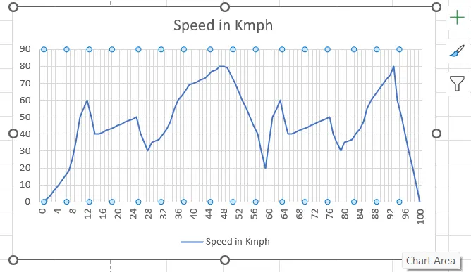
| No. | Initial Velocity (km/h) | Final Velocity (km/h) | Time Required (s) | Deceleration (m/s²) | Energy Required (J) | Braking Power (W) | Braking Energy (Wh) |
|---|
| 1 | 60 | 40 | 3 | 1.85 | 277,778 | 92,592.6 | 25.7 |
| 2 | 50 | 30 | 3 | 1.85 | 222,222 | 74,074.1 | 20.6 |
| 3 | 80 | 20 | 11 | 1.52 | 833,333 | 75,757.6 | 21.0 |
| 4 | 60 | 40 | 3 | 1.85 | 277,778 | 92,592.6 | 25.7 |
| 5 | 50 | 30 | 3 | 1.85 | 222,222 | 74,074.1 | 20.6 |
| 6 | 80 | 0 | 7 | 3.17 | 888,889 | 126,984.1 | 35.3 |
| Total Braking Energy Required (Wh) | 148.9 | | |
This method provides an estimate of the energy required for braking, considering both mechanical dissipation and potential energy recovery.
===============================================================================================================
2.Why electric motor can’t develop braking torque at high speed similar to starting? How electric and mechanical brakes are coordinated?
An electric motor’s ability to generate braking torque at
high speeds differs from its ability to generate starting torque due to the
following reasons:
- Back
Electromotive Force (Back-EMF)
- At
high speeds, the motor generates a significant back-EMF, which opposes
the applied voltage and limits the current available for braking. Since
braking torque is directly proportional to current, the available torque
decreases.
- Field
Weakening at High Speed
- Many
electric motors (especially induction and PMSM motors) use field
weakening beyond the base speed. This reduces the magnetic field
strength, which in turn lowers the available braking torque at high
speeds.
- Regenerative
Braking Limitations
- In
regenerative braking, the motor acts as a generator, converting kinetic
energy into electrical energy. However, at very high speeds, the power
electronics and battery may not be able to handle the high voltage
generated, limiting regenerative braking capability.
- Inverter
and Power Electronics Constraints
- The
inverter controlling the motor has operational limits on voltage and
current. At high speeds, voltage saturation can occur, preventing the
motor from developing sufficient braking torque.
- Torque-Speed
Characteristics
- Motors
provide high torque at low speeds (constant torque region) but have
reduced torque in the high-speed range (constant power region). This
affects braking performance, just as it affects acceleration.
Electric and mechanical brakes are coordinated through brake
blending to ensure efficient, smooth, and safe deceleration. The coordination
process involves:
- Regenerative
Braking Priority
- The
system first prioritizes regenerative braking to recover energy and
recharge the battery.
- Transition
to Mechanical Brakes
- If
the required braking force exceeds the regenerative braking capability
(e.g., at low speeds or during emergency braking), mechanical brakes
(friction brakes) supplement the braking effort.
- Brake
Control System (Blending Algorithm)
- A Brake
Control Unit (BCU) or Vehicle Control Unit (VCU) continuously monitors
speed, driver input, and braking torque demand to distribute braking
force between the motor and mechanical brakes.
- ABS
and Stability Control Integration
- Mechanical
brakes provide higher reliability in emergencies and are necessary for
ABS (Anti-lock Braking System) and stability control, which operate
independently of regenerative braking.
- Creep
Mode and Low-Speed Braking
- At
very low speeds, regenerative braking becomes ineffective, so mechanical
brakes fully take over to bring the vehicle to a complete stop.
================================================================================================================
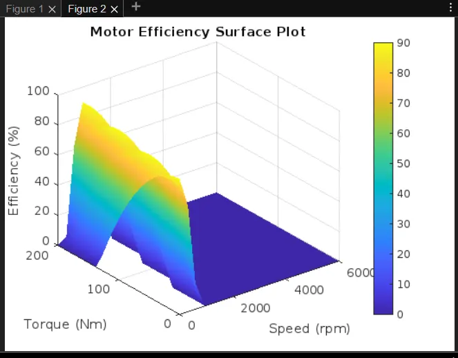
3.Make a MATLAB program which plots contour of given motor speed, torque and efficiency values. Attach the code as a .m file attach a screenshot of all the plots.
% MATLAB Program to Plot Motor Efficiency Contour
% Define Speed (rpm) and Torque (Nm) Ranges
speed = linspace(0, 6000, 20); % Speed from 0 to 6000 rpm
Torque = linspace(0, 200, 20); % Torque from 0 to 200 Nm
% Create Meshgrid
[torqueGrid, speedGrid] = meshgrid(Torque, speed);
% Define Efficiency Function (Example Model)
efficiency = 90 - (0.0002 .* speedGrid.^2) - (0.005 .* torqueGrid.^2) + (0.002 .* speedGrid .* torqueGrid);
efficiency(efficiency < 0) = 0; % Ensure efficiency is non-negative
efficiency(efficiency > 100) = 100; % Limit efficiency to 100%
% Plot Contour Map
figure;
contourf(speedGrid, torqueGrid, efficiency, 20);
colorbar;
xlabel('Speed (rpm)');
ylabel('Torque (Nm)');
title('Motor Efficiency Contour Plot');
grid on;
% Save Contour Plot
saveas(gcf, 'motor_efficiency_contour.png');
% 3D Surface Plot
figure;
surf(speedGrid, torqueGrid, efficiency);
colorbar;
shading interp;
xlabel('Speed (rpm)');
ylabel('Torque (Nm)');
zlabel('Efficiency (%)');
title('Motor Efficiency Surface Plot');
grid on;
% Save 3D Plot
saveas(gcf, 'motor_efficiency_surface.png');
OUTPUT :
Figure 1
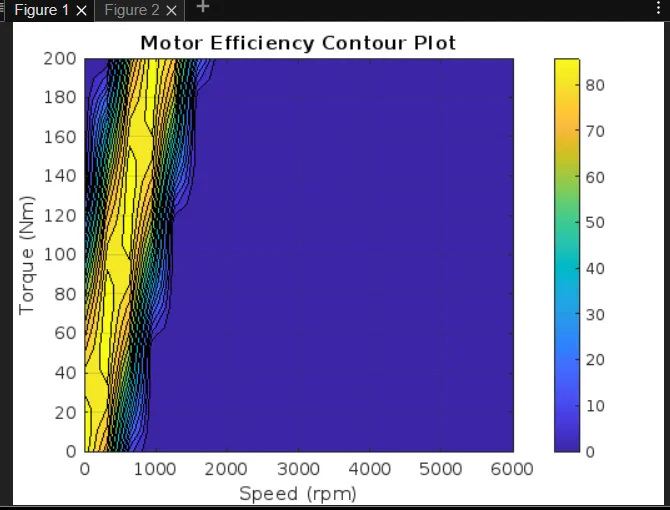
figure 2
======================================================================================================================