Week-11 Challenge: Braking

Q1. For a defined driving cycle, calculate the energy required for braking.

Calculating the energy required for braking of HWFET Drive Cycle-

Braking: Braking is a condition to slow down or stops a moving vehicle as required. There are several techniques to
apply brakes, which can be mechanical or electrical. The most commonly used technique is by applying friction. It consumes energy .The consumed kinetic Energy can be derived as following equation-

Braking Energy = (1/2) *m*v^2

Where, Braking Energy is the kinetic energy in unit of Joule.
M = Total Mass of the Vehicle (Vehicle Mass + Pay Load) in unit of Kg.
V = (Initial Velocity-final Velocity) in unit m/s.

For Example if Initial speed of a vehicle is 20m/s and final speed is 10m/s. The mass of the vehicle is 500kg. Then the
required kinetic energy for Braking is (1/2)*500* (20-10)^2 = 25000 J =25KJ.

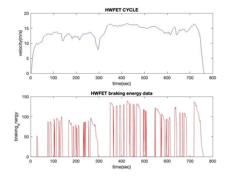
Here for a Drive cycle the required braking energy is calculated for each second of time to slow down or stop the vehicle- Braking Energy Calculation for HWFET Driving Cycle.

Plot :

clear all
close all
clc

% Given parameters and importing the given file
HWYCOL = xlsread('HWYCOL.xlsx');                % import HWFET data cycle
kW = 2000;                                      % assuming the Kerb Weight
PL = 0.5 * (2000);                              % assuming the Pay load 
TM = kW + PL;                                   % assuming the total mass parameters
g  = 9.81;                                      % acceleration due to gravity
time = HWYCOL(:,1);                             % taken the values of all row os first coloumn should be consider as time
velocity = HWYCOL(:,2);                         % taken the values of all row of second coloumn should be consider as velocity
speed = (velocity).* 0.2778;                    % convert velocity kmph to mps
Ibe=zeros(1,length(time));                      % Ibe is instant braking energy

for i = 1:(length(velocity)-1)                  % creating the values if 1369 values for equation
    if speed(i)>speed(i+1)                      % from the formula assign the statement as final value is always less then initial value 
       Ibe(i) = 0.5 * TM * 0.001 * (speed(i)).^2 - (speed(i+1)).^2; % applying braking energy formula
    end   
end

% plotting

subplot(2,1,1)
plot(time,speed,'Color','B')
xlabel('time(sec)')
ylabel('velocity(m/s)')
title('HWFET CYCLE')
subplot(2,1,2)
plot(time,Ibe,'Color','R')
xlabel('time(sec)')
ylabel('braking_energy')
title('HWFET braking energy data')

Plotting :

Q2. Why electric motor can’t develop braking torque at high speed similar to starting? How electric and mechanical brakes are coordinated?

This situation occurs only when the vehicle is at high speeds because the motor will be running at the constant power region. In the constant power region, the torque of the motor reduces and so the motor cannot develop the braking torque which is equal to the torque that occurred during low speed at the constant torque range.

The torque vs speed plot of a vector control induction motor is given below.

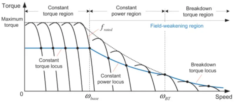
From the above characteristic curves of the motor. that is seen that the torque of the motor remains high at low speeds and reduces as the speed increases.

Since the electric motor cannot develop braking torque at a high speed similar to starting.

Electrical brake and mechanical brake.

Electrical braking

Electrical braking can be done by many methods such as,

• Unbalancing the input points of current to the motor.
• Using transistors in H-bridge arrangement to reverse the motor direction in order to reduce speed.
• Implementing a regenerative braking system by using bidirectional power converters.
• Regenerative braking converts much of the energy to electrical energy, which may be collected for later use.

Mechanical braking

Mechanical brakes commonly use friction between two surfaces pressed together to convert the kinetic energy of the moving object into heat, though other methods of energy conversion may be employed. The friction between the surfaces is performed using pressurized air or pressurized oil which are commonly known as an air brake and hydraulic brake respectively.

Coordination of electrical and mechanical braking in EV's

Two types of brake control strategies are used to organise the electrical brake and mechanical brake they are,

• Series control strategy
• Parallel control strategy

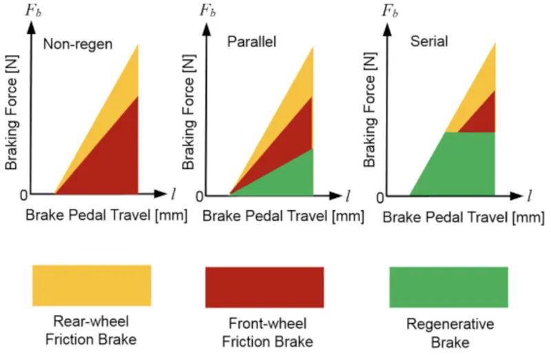
The comparison of the control strategies is shown in the below figure.

In the figure, it is seen that, according to the amount of brake pedal travel of the vehicle, the mechanical brakes and regenerative brake are employed.

Parallel control strategy

When the brake is applied according to the brake pedal travel the front wheel friction brake, the rear wheel friction brakes and the regenerative brakes are employed simultaneously. The higher the travel of the brake pedal the higher the amount of braking will be done.

The braking energy is distributed in the following practice,

Rear-wheel friction brake ----› Front-wheel friction brake ----› Regenerative brake

Series control strategy

When the brake is applied according to the brake pedal travel the front wheel friction brake, the rear wheel friction brakes and the regenerative brakes are applied one after another. As the braking requirement increases the frictional brakes are used subsequently.

For low speeds of the vehicle, regenerative braking is used but it may be limited according to the Soc (state of charge) of the battery.

As the speed of the vehicle increases the rear wheel frictional brake will be employed if the braking requirement is not done but then the front wheel frictional brake is also used.

The coordination of the series control braking can be done with the choice to the comfort of braking (or) energy storage.

Electric driven intelligent brake (EDIB)

EDIB is a brake control strategy which is developed by NISSAN. It is a type of parallel braking which can be seen in the
below image.

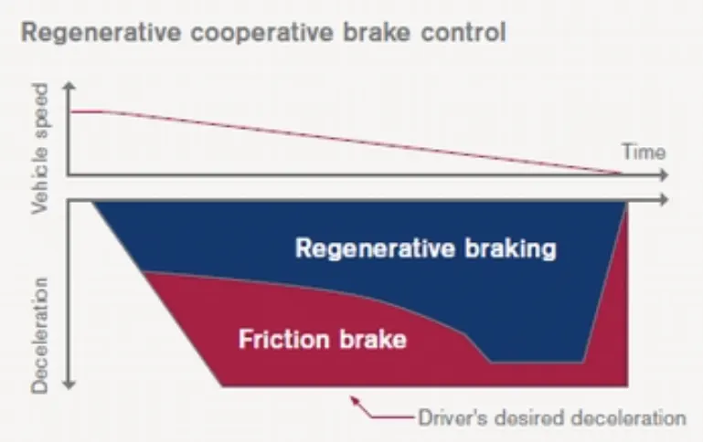
The above image shows that the frictional brake and the regenerative brake are used simultaneously at higher speeds of the vehicle.

At low speed the torque of the motor is high and so the regenerative brake has a higher braking part than the frictional brakes.

Brief working of EDIB

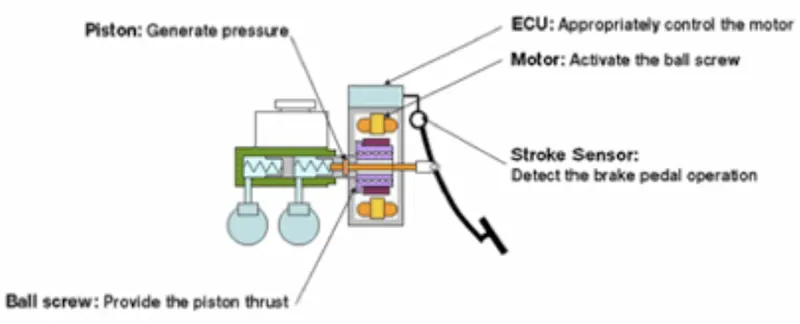
When the driver steps on the brake pedal, the stroke sensor detects the operation of the brake. That report is communicated to the ECU and controls the motor. The motor engages the piston through the ball screw and increases the friction brake's pressure (hydraulic pressure). Through optimum control of the friction brake's hydraulic pressure, the energy regeneration result is maximized.

Q3. Make a MATLAB program which plots contour of given motor speed, torque and efficiency values. Attach the code as a .m file attach a screenshot of all the plots.

clear all
close all
clc

% Speed Array
omega = linspace(0, 300, 100) ;

% Torque Array
T = linspace(0, 2000, 100) ;

% Meshgrid
[X,Y] = meshgrid (T, omega) ;

% Loss Coefficients
cu = 0.17;                      % Copper coefficient
fe = 0.006;                     % Iron coefficient
win = 0.000015;                 % Windage coefficient

% Losses
cu_loss = cu*(Y.^2);            % Copper Losses
fe_loss = fe* (X.^2);           % Iron Losses
win_loss = win*(X.^3);          % Windage Losses
cond_loss = 18;                 % Conduction Losses

% Output Power
P_out = (X.*Y);

% Input Power
P_in = P_out + (cu_loss) + (fe_loss) + (win_loss) + (cond_loss);

% Efficiency
n = ( (P_out)./ (P_in)) ;

% Efficiency values for contour
W= linspace (0.75, 0.95, 10);

% Contour Plot
contourf(X, Y,n, W)
colorbar
xlabel ('Angular Speed, rad/s')
ylabel( 'Torque, Nm' )
title('Speed, Torque and Efficiency characteristics of Motor')

Explanation:

In this MATLAB script, we create arrays for the speed and the torque of the motor using the 'linspace' command. For the speed, consider a range of values from 0 to 2000 radians per second whereas for the torque, consider a range of values from 0 to 300Nm.These arrays are then used to create 2D grid coordinates using the 'meshgrid' command. These coordinates will help in the creation of the contour plot. In order to find the efficiency of the motor, we need to consider the various losses that occur in the motor's operation. These are:

• Iron losses
• Schedule Now
• Windage losses
• Conduction losses

These various losses are dependent on the speed and the torque of the motor. They each also have a characteristic constant of proportionality which are all assumed for the following calculations and represented as 'K'. In each calculation, the speed and the torque are represented respectively as: w and T.

Copper losses = KCu•02

Iron losses =KFe•T2

Windage losses =KW• T3

The values of coefficients are taken as general values. Conduction losses are assumed to be 18 Joules.

Finally we plot the contour with the 'contour' command. In addition, an array for the efficiency values we want to plot for is created called W' and is assigned for values ranging from an efficiency level of 0.75 to 0.95. This array is used in the creation of the contour. Axis labels and a title is also made for better readability.

Output :

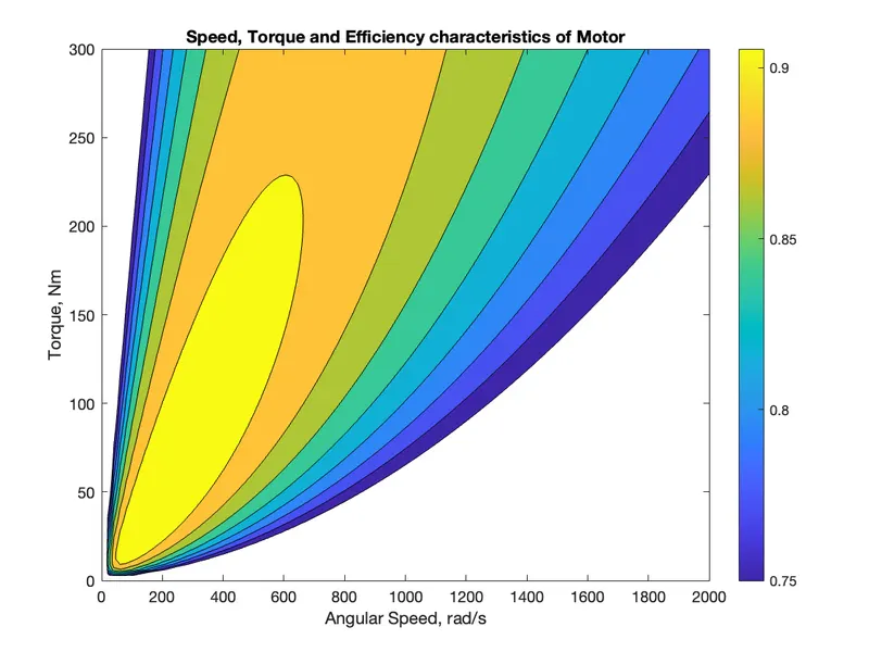
From the Inner Most Plot, We can Find that efficiency arises in innermost point of the contour plot and this efficiency decreases as the Contour Plot increases in size from inntermost contour plot.