Week-11 Challenge: Braking
For a defined driving cycle, calculate the energy required for braking.
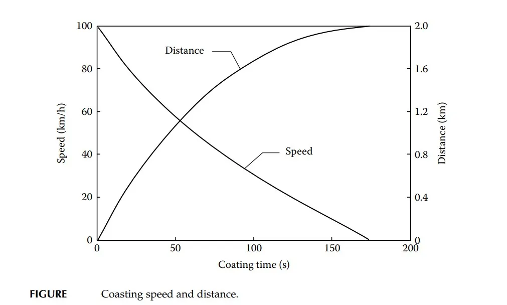
A significant amount of energy is dissipated by braking.1–3 Braking a 1500- kg vehicle from 100 km/h to zero speed dissipates about 0.16 kWh of energy [(1/2)MV2] in a few tens of meters. If this amount of energy is dissipated by coasting and only by drag forces (rolling resistance and aerodynamic drag) without braking, the vehicle will travel about 2 km, as shown in Figure below.
When a vehicle is driving in a stop-and-go pattern in urban areas, a significant amount of energy is dissipated by frequent raking. Successful design of the hybrid braking system for recovering as much of the braking energy as possible requires a full understanding of braking behavior and its characteristics with respect to vehicle speed, braking power, deceleration rate, and so on during typical urban driving cycles
While driving on a flat road, the driving power on the vehicle wheels can be calculated by
`P_d=V/1000 (M〖gf〗_r+1/2 ρ_a C_d AV^2+Mδ dV/dt) (kW)`
→ 1
where M is the vehicle mass in kg, g is the gravitational acceleration, 9.81 m/s2, fr is the tire rolling resistance coefficient, ρa is the air mass density, 1.205 kg/m3, CD is the aerodynamic drag coefficient, A is the frontal area of the vehicle in m2, V is the vehicle speed in m/s, δ is the rotational inertia factor, and dV/dt is the vehicle acceleration in m/s2 (and is negative for deceleration). For Pd > 0, the traction wheels accept power from the power plants and push the vehicle forward. In this case, the braking power is zero. In contrast, Pd < 0 when braking and the kinetic energy of the vehicle mass is dissipated by the brake system. In this case, the driving power is zero. Integrating Equation 1 over the driving time in a given driving cycle can give both the traction energy and braking energy, as shown in Figure (a) for a typical passenger car with the parameters listed in Table 1(a) in the FTP75 urban driving cycle.
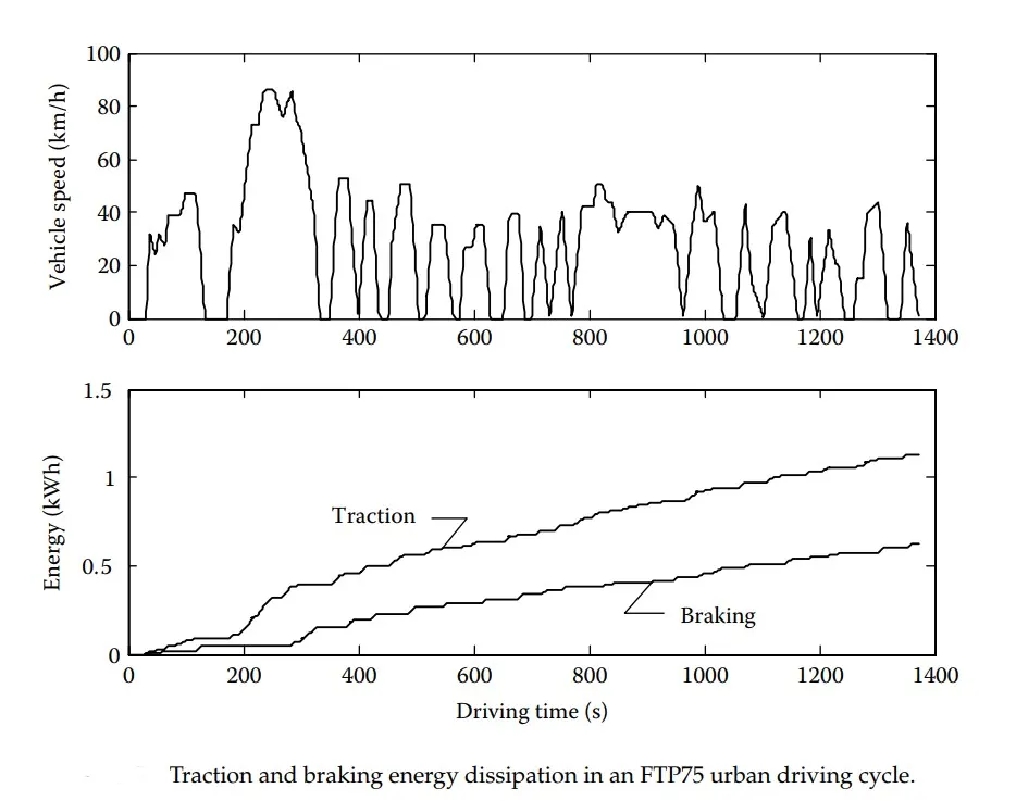
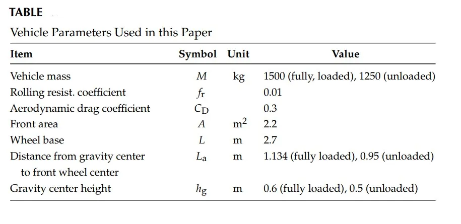
The vehicle parameters used in this are shown in Figure (b) and Table 1(a).
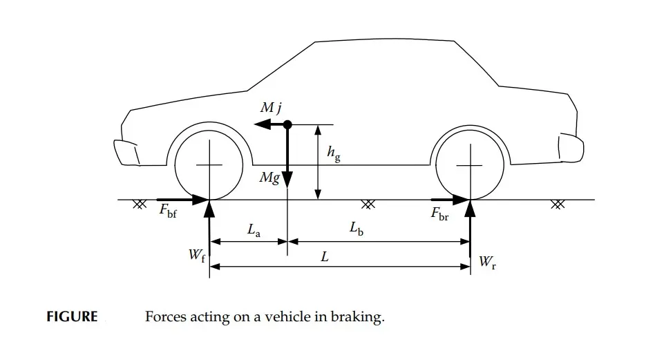
Figure (b) and Table 1(b) indicate that the braking energy in typical urban areas may reach up to more than 34% of the total traction energy. In large cities, such as New York City, it may reach up to 80%.
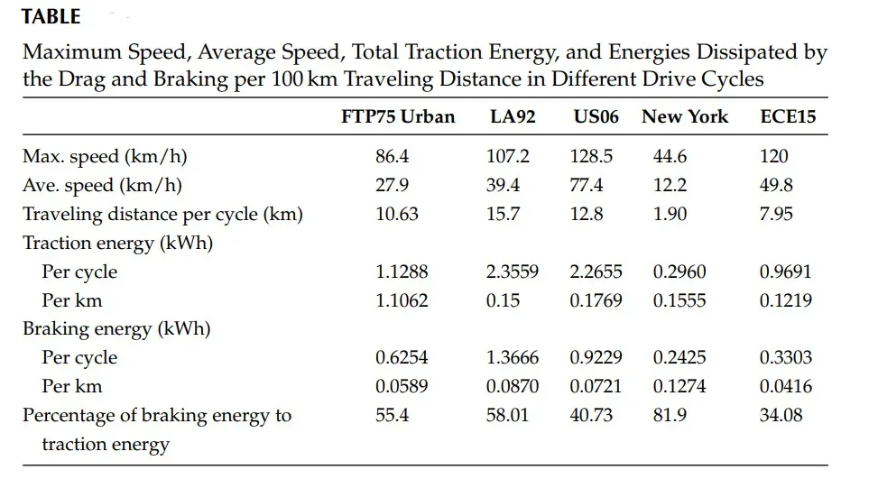
Figure (b) and Table 1(b) indicate that the braking energy in typical urban areas may reach up to more than 34% of the total traction energy. In large cities, such as New York City, it may reach up to 80%.
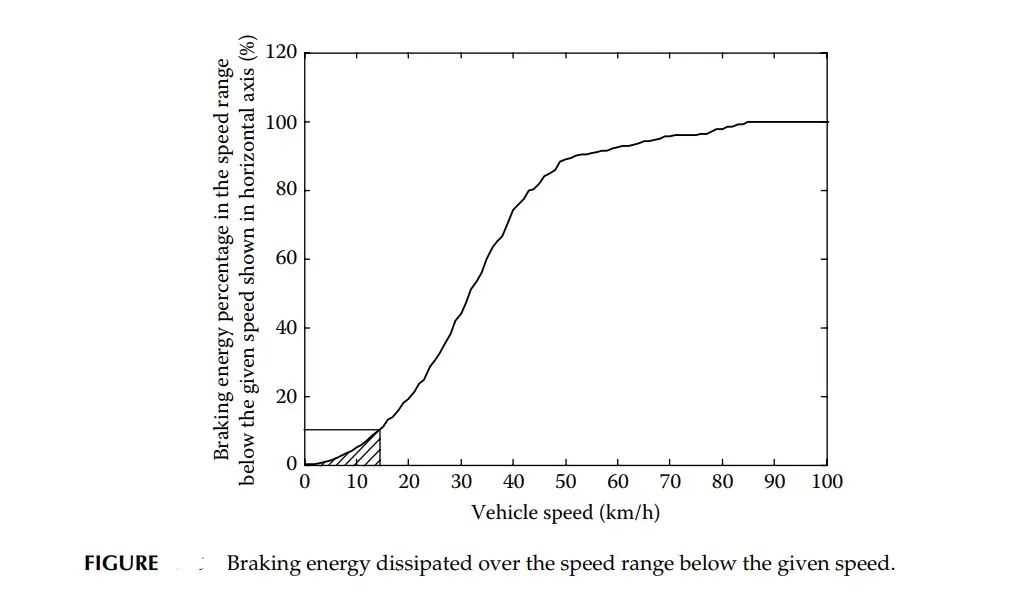
Table 1(c) shows the braking energy dissipated in the speed range below 15 km/h while driving in other typical urban driving cycles.
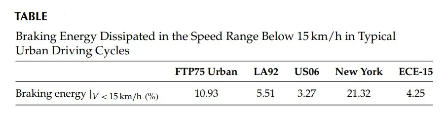
The braking energy dissipated in the low-speed range, such as below 15 km/h in all the typical driving cycles, is insignificant. This result indicates that we need not attempt to obtain high operating efficiency at low speeds in the design and control of regenerative braking. In fact, it is difficult to regenerate at low speeds, because of the low motor electromotive force (voltage) generated at low motor rotational speeds. It should be noted that the rotational speed of the vehicle driven wheels, which is proportional to motor angular speed, is decoupled from the translatory speed of the vehicle body when the vehicle wheels are close to being locked. Thus, the operation of the hybrid brake system must be at speeds higher than a minimum threshold value. Electric regenerative braking should be applied primarily to recapture as much braking energy as possible. At speeds lower than this threshold, mechanical braking should be primarily applied to ensure the vehicle’s braking performance.
Why electric motor can’t develop braking torque at high speed similar to starting? How electric and mechanical brakes are coordinated?
In a motor torque-speed characteristics there are 2 regions
1.Constant torque region
2.Constant power region
At high speeds the motor characteristics is in the constant power region, when the brake torque is applied, it will not be as much as in the starting speed, because the as the rate of charge is less than the rate of discharge.
In induction motor at high speed the synchronous speed is more than the motor speed, so the braking torque will be less, as the braking torque is applied when the motor speed is more than the synchronous speed as in the starting speed.
At the start speed the motor torque will be matching the load torque,where as the in high speed the torque will also be matching unless the brake is applied or the voltage supply is cut the load torque will be more than the motor torque hence the brake torque is less and delayed braking.
Coordination of electric and mechanical brakes.
Figure 1 shows a braking force allocation strategy, in which the mechanical brake has a fixed ratio of braking force distribution on the front and rear wheels represented by the β line. Curve I is the ideal braking force distribution of the vehicle. The ECE regulation, which stipulates the minimum rear braking force, is also plotted. The total braking force is the curve labeled mechanical + electrical. The braking force on the front wheels consists of mechanical braking, Fbf-mech ,and electric braking, Fbf-regen, as shown in Figure 13.10. When the wheel speed is lower than given threshold, 15km/h for example, either very low vehicle speed or speed close to wheel lock-up,the electric regenerative braking will produce no braking force and the braking is completely done by the mechanical system.
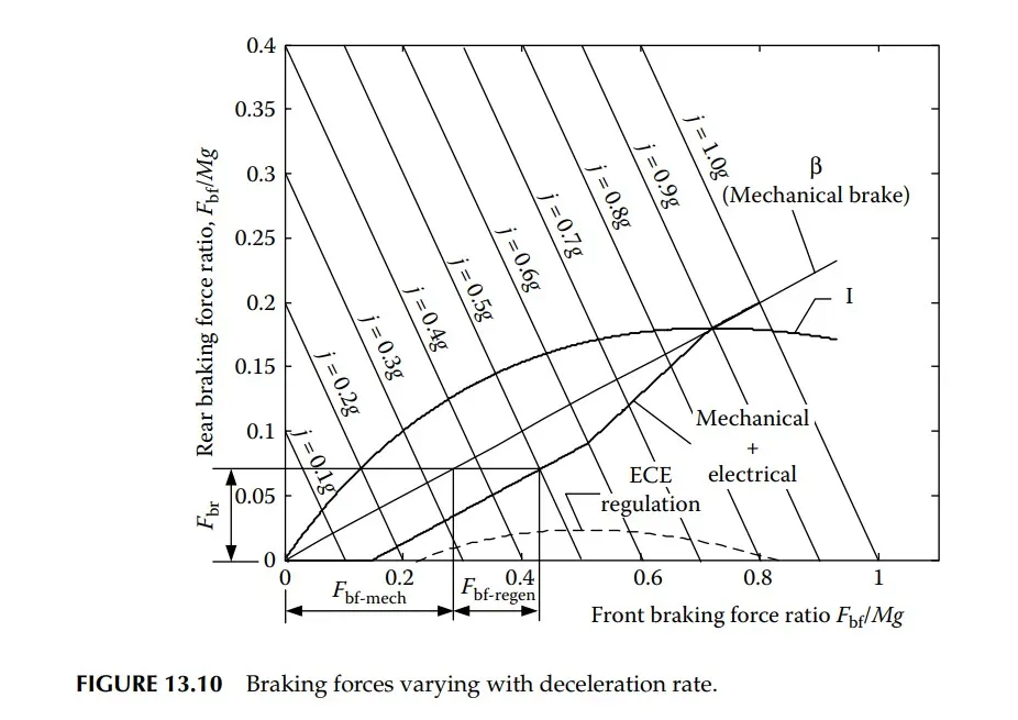
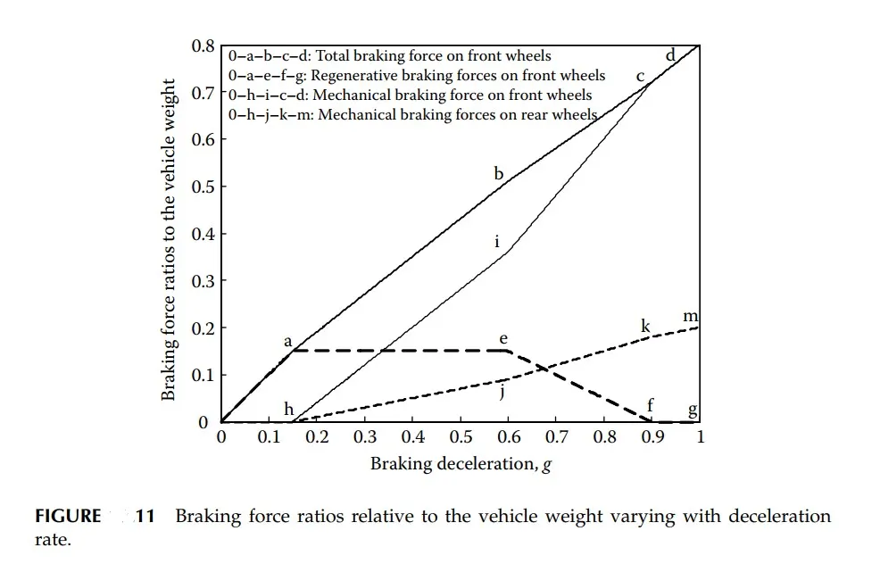
When the wheel speed is higher than the given threshold and the desired vehicle deceleration is less than a given value (0.15g in Figure 13.10), which is represented by the stroke of the brake pedal, all the braking force is produced by electric regenerative braking and no mechanical braking force is applied to the front and rear wheels. Zero mechanical force may be implemented by employing larger clearances between the brake pads and plates or by carrying out small modifications to the conventional master cylinders. When the desired deceleration is greater than the given value (0.15g in Figure 13.10), both mechanical and electric braking share the total front wheel braking force as shown in Figure 13.10. The design of the electric braking portion is associated with the power capacity of the electric motor and on board energy storage. But the total braking force curve in Figure 13.10 must be above the ECE regulation curve. When the desired deceleration is higher than a given value (0.6g in Figure 13.10), the electric regenerative braking force is gradually reduced to zero with increase of the desired deceleration (0.9g in Figure 13.10). This design will ensure that the actual front and rear wheel braking forces are close to the ideal braking distribution curve, resulting in short braking distances, and strong mechanical braking that may be more relied upon for emergency cases. Figure 13.11 shows the total braking force, regenerative braking force, and mechanical braking forces on the front and rear wheels, respectively, along with vehicle deceleration rate.
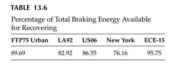
With the design principle described above and the electric regenerative braking control rule with respect to wheel speed, the braking energy available for recovering can be computed in various typical driving cycles by using a computer model. The simulation results are listed in Table 13.6. The data indicate that in normal urban driving, most of the braking energy can be recovered. It should be noted that the maximum braking torque required of the electric motor is that which can produce 0.15g of deceleration. Thus, a large-sized electric motor would not be needed.
%x axis corresponds to motor speed (w)
%y axis to the Torque (t)
x = linspace(1,1000); %N.B speed rad/s nit in rpm
y = linspace(1,250); %0 to 40 N-m
%motor loss constants
kc=0.2; %copper loss constant
ki = 0.008; %iron losses constant
kw = 0.0001; %windage losses constant
ConL = 20; %constant motor losses
[X,Y] = meshgrid(x,y);
outputpower = (X.*Y); %torque*speed = power
B = (Y.^2)*kc; %copper losses
C = X*ki; % iron losses
D = (X.^3)*kw; %windage losses
inputpower = outputpower+B+C+D+ConL;
Z = outputpower./inputpower;
%we now set the efficiency values foe which contours willl be plotted
V = [0.7 0.8 0.85 0.9 0.91 0.92 0.925 0.93];
box off
grid off
contour(X,Y,Z,V);
xlabel('Speed rad./s^-^1')
ylabel('Torque /N-m')
hold on
%now plot a contour of the power output
%The array ouptut Power has already been calculated
%we draw contours at 3 and 5 kw
V=[8000,10000];
contour(X,Y,outputpower,V);
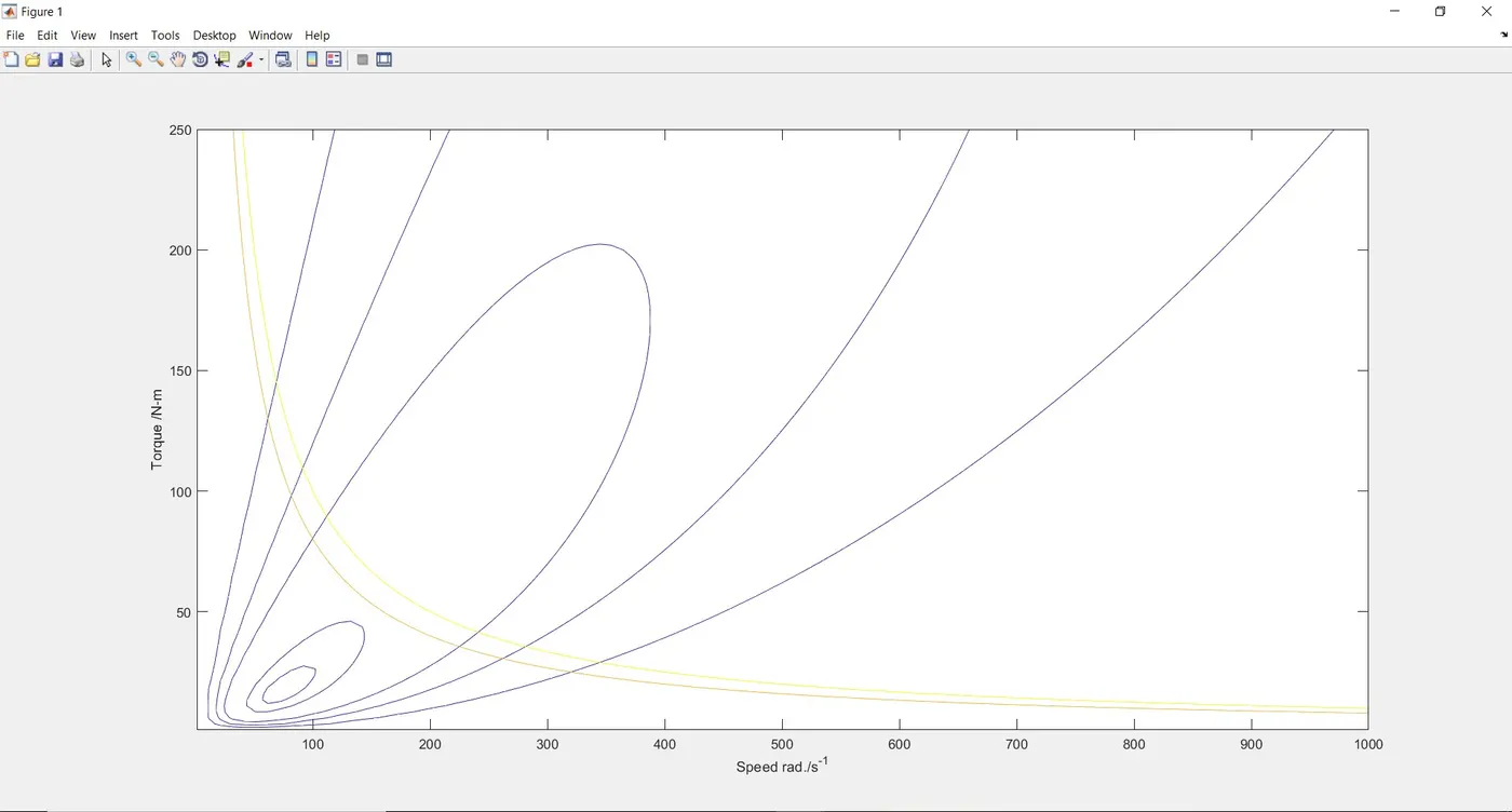
The output plot of the above matlab code: