Week 10 - Validation studies of Symmetry BC vs Wedge BC in OpenFOAM vs Analytical H.P equation

Note:This challenge is a continuation of week 11 challenge

In this challenge you will simulate the same problem as in week 1 but by applying Symmetry Boundary Condition.You will do the simulation for the below mentioned angles using both Symmetry and Wedge boundry conditions and validate them with HP equation like you did in week 11 challenge.

Angles to test

*10⁰

*25⁰

*45⁰

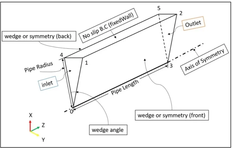
:-Axi-Symmetric geometry using the wedge patch type .

Selection key Description

Pateh generic patch

Symmetry plane of symmetry

Empty front and back planes of a 2D geometry

Wedge wedge front and back for an axi-symmetric geometry

Cyclic cyclic plane

Wall wall-used for wall functions in turbulent flows

Processor inter-processor boundary

:- Bose types

The bace and geometrics types are described below,the keywords used for specifying types in OpenFOAM

:-Basic patch types.

:-Patch

the basic patch type for condition that no gemetric or topological information about the mesh (with the exception of wall) ,e.g an inlet or an outlet.

:- Wall

There are instances where a patch that coincides with a wall need to be identifiable as such , particularly where specialist modelling is applied at wall boundaries .A good example is turbulence modelling where a wall must be specified with a wall patch type, so that the distance form the wall of the cell centers next to the wall are stored as part of the patch.

:-symmetry plane.

for a symmetry plane.

:- Empty

While Open Foam always generates geometries in 3 Dimensions ,it can be instructed solve in 2 or 1 dimensions by specific a special empty condition on each patch whose plane is normal is normal to the 3rd and 2nd dimension for which on solution is required.

:-Wedge

For 2 Dimensional axi-symmetric cases, a cylinder,the geometry is as a wedge of small angel(eg.<5\relax\special)and 1 call thick running along the plane of symmetry,saddling one of coding pleas ,as show in .The axi-symmetric wedge planes must be specified as spare patches of wedge type.The details of generating wedge-shaped geometric using block mesh are described in section .

:-cyclic

Enables two patches to be treated as if they are physically connected; used for repeated geometries e.g. heat exchange tube bundles .one cycle patch is linked to another through a neighborliness keyword in the boundary file.

each pair of connecting must have similar area to within to tolerance given by the match Tolerance keyword in the boundary file.Faces do not need to be same orientation.

:-processor

if a code is being run in parallel , on number of processors, then the mesh must be divided sothat each processor computes on roughly the same number of cells. The boundaries between the different parts of the mes are called processor boundaries.

SIMULATION PROCEDURE:-

Problem setup:-

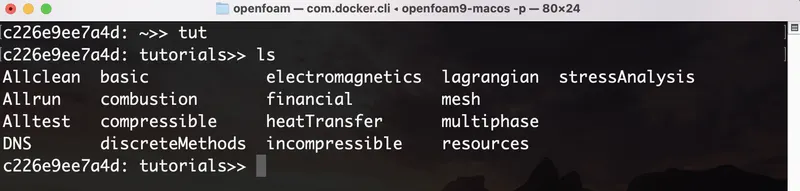
We firs initialize the problem by navigating to the tutorials directory by OpenFoam by usinf the "tut" command in the terminal window. From the tutorials ,we have to figure out the suitable case files for our given problem, which is an axi -symmetric laminar flow through a constant cross section pipe. We use "ls" command to list the contents files or directories present inside the directory.

As it is an incompressible flow, we navigate into the incompressible directory. WE use the "cd" command to navigate and change the working directory using the terminal window.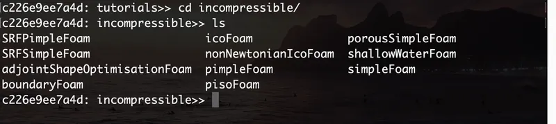

The next step involves navigating into the iocFoam directory ,as the type of colver for this problem is icofaom . the iocfoam command solves the incompressible laminar navies-srockes equations. This code inherently transient,eruiring an initial condition such as zero velocity and boundary conditions.

Here ,we use the cavity utility to create our required domain . We copy this directory into the FOAMRUNfile,wnichisadefaultfileOpenFoamcreatesfoeus.Weuse"cpr"commandtorecursivelycreatyofthecontentsofthefileordirectoryintothe$FOA{M}_{R}UNfile,wnichisadefaultfileOpenFoamcreatesfoeus.Weuse"c{p}_r"commandtorecursivelycreatyofthecontentsofthefileordirectoryintothe$FOAM_RUN folder undwer the file name "Flow Through pipe" for personal use .We create a copy of the files as OpenFoam does not let us modify or make changes to its inbuilt tutorial files.

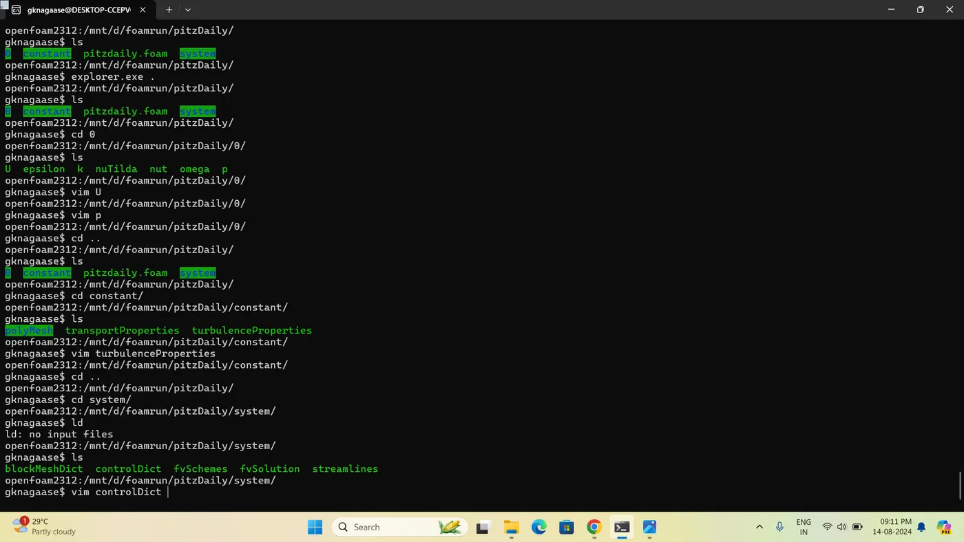
we then navigate to the copies tutorial file in $FOAM_RUN directory to view the contents inside the folder.

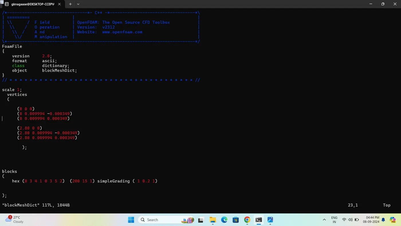
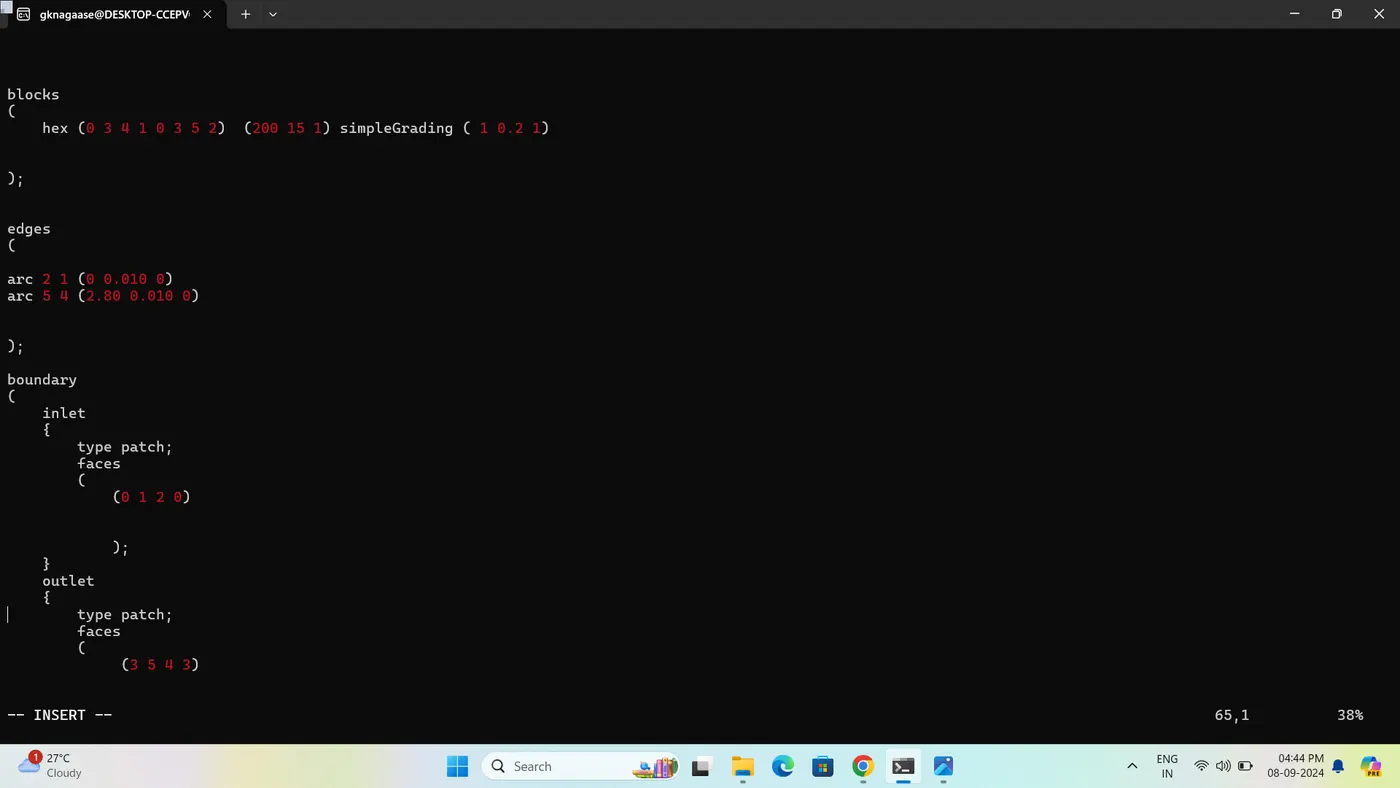
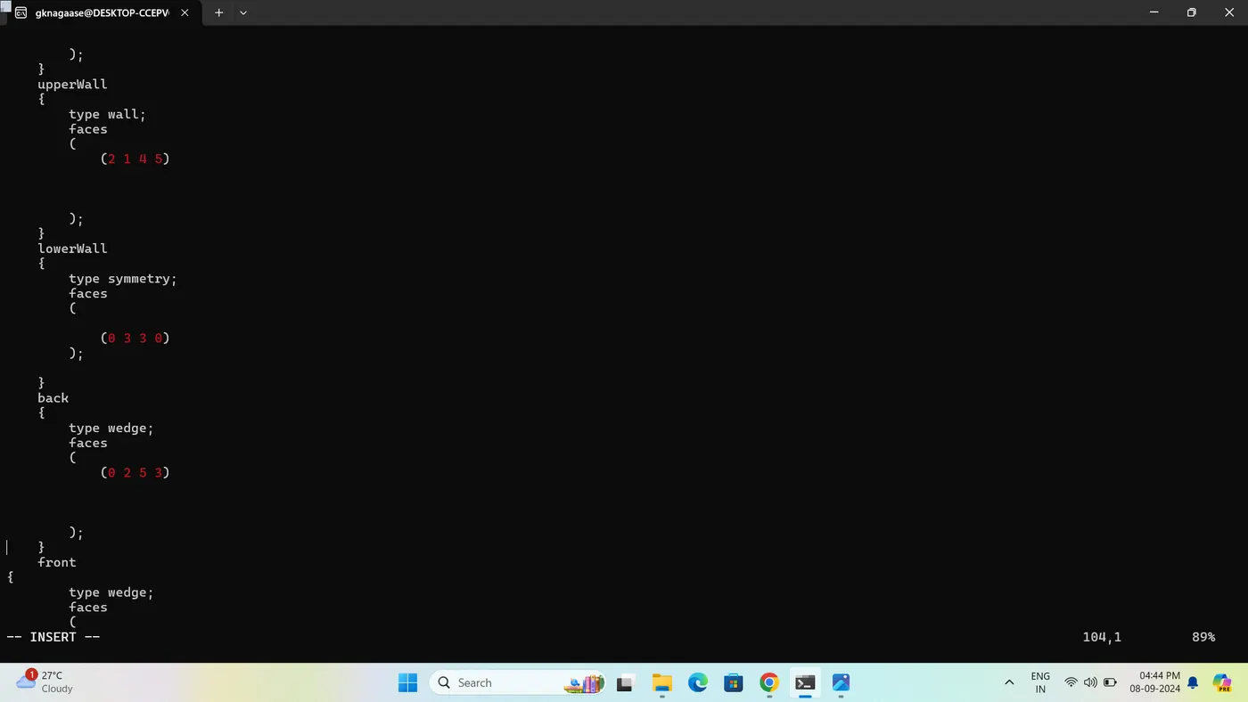
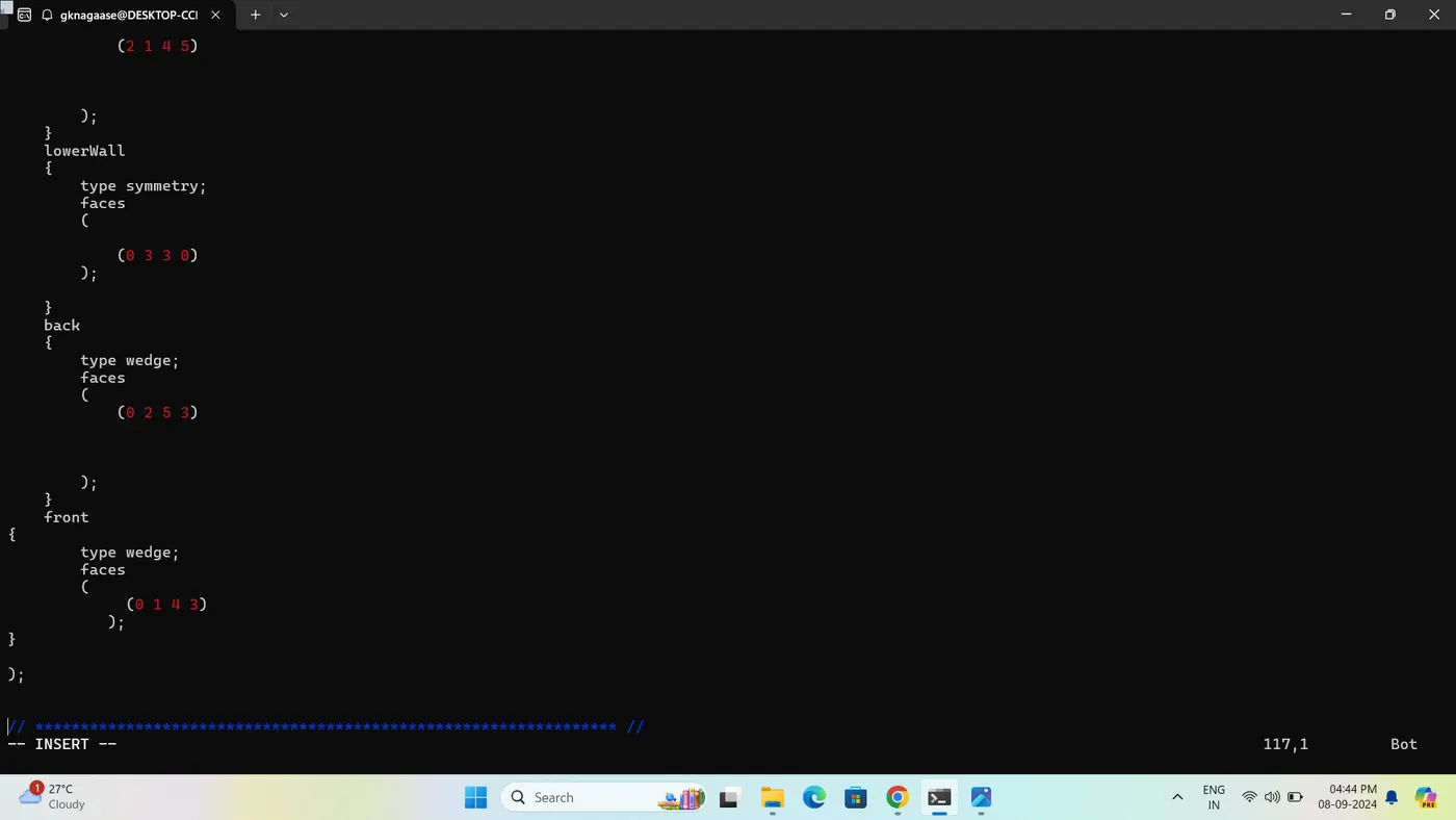
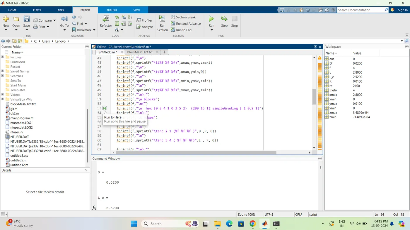
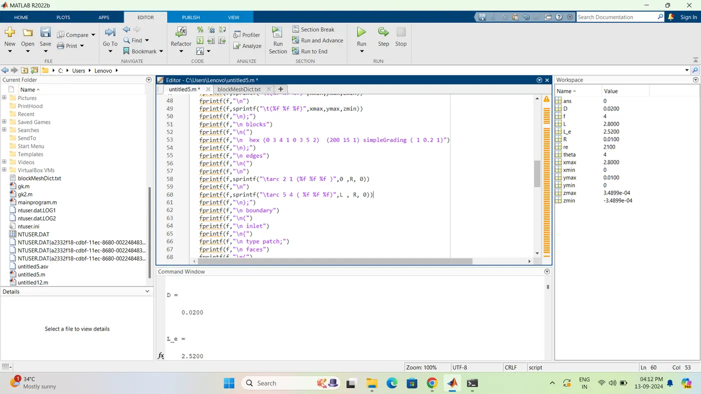
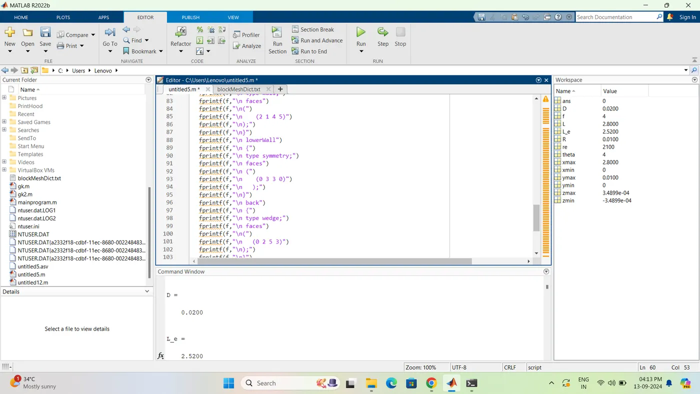
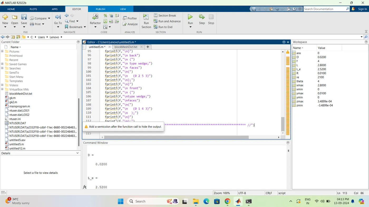
Matlab Program :-

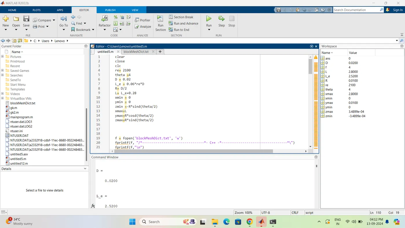
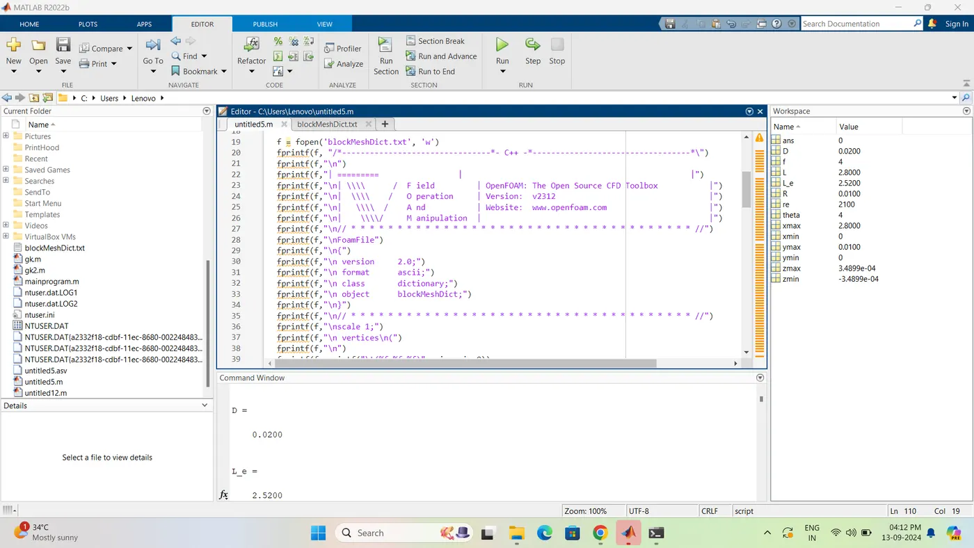
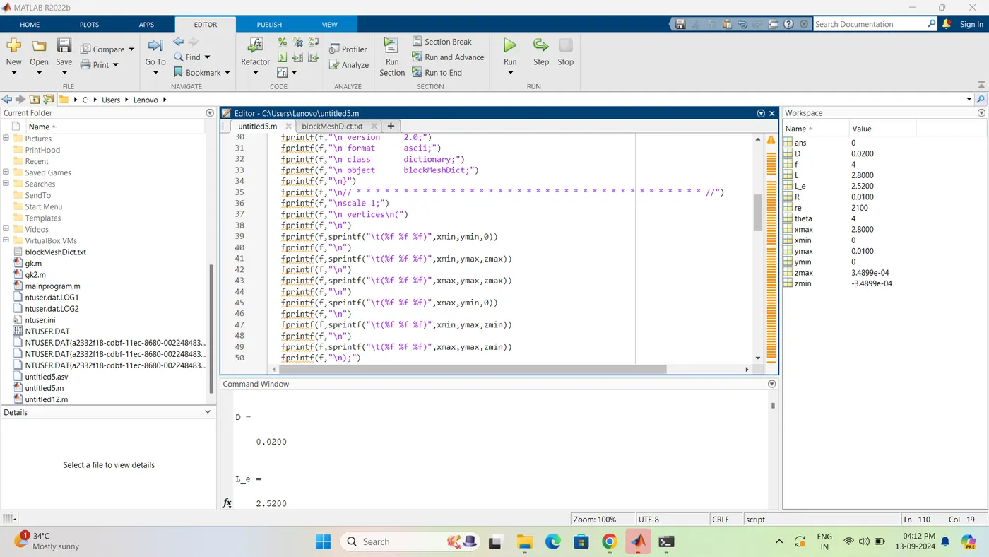
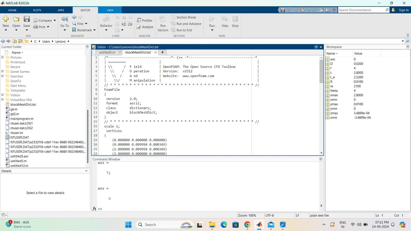
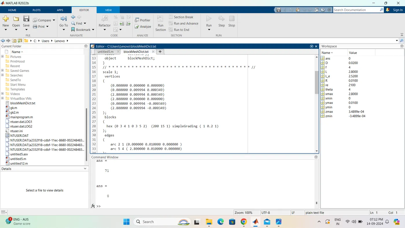
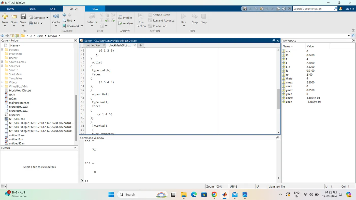
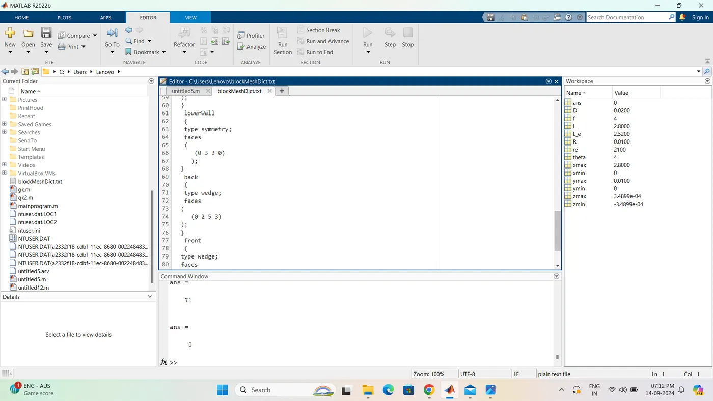
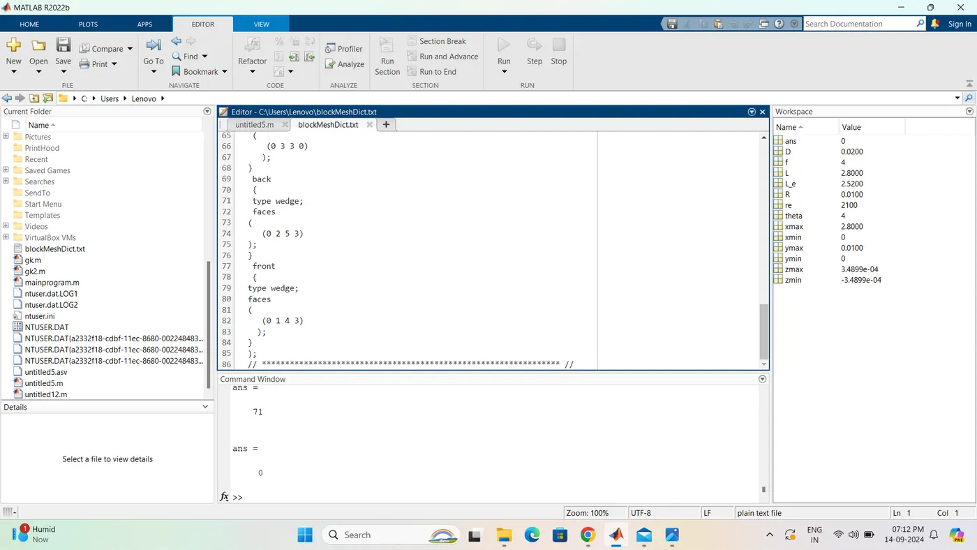
Output of program Geometry:-

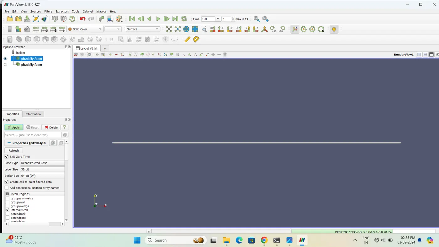
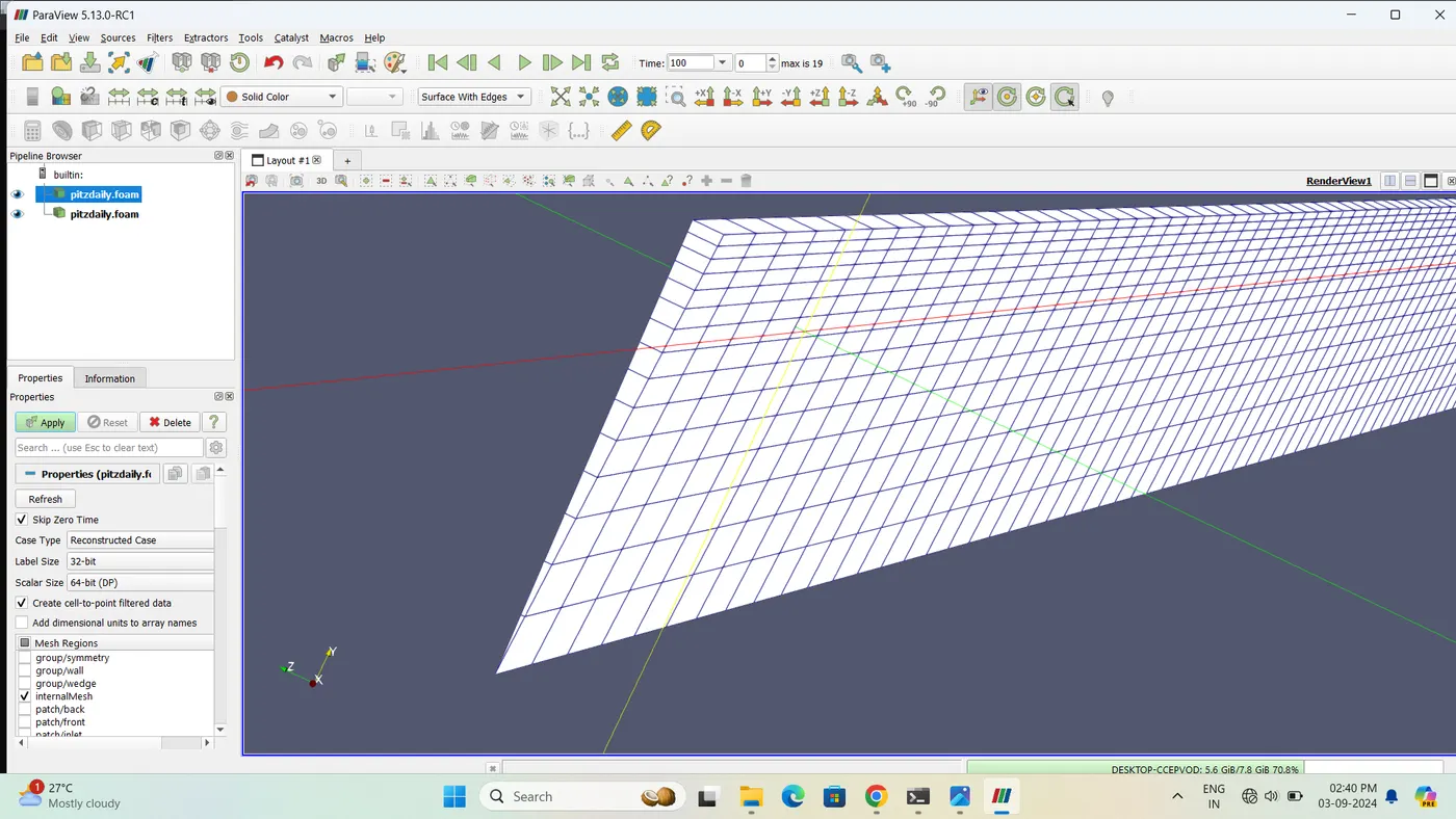
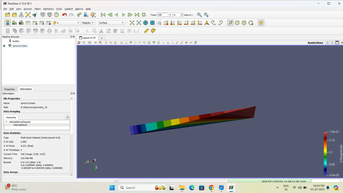
open in para View:-

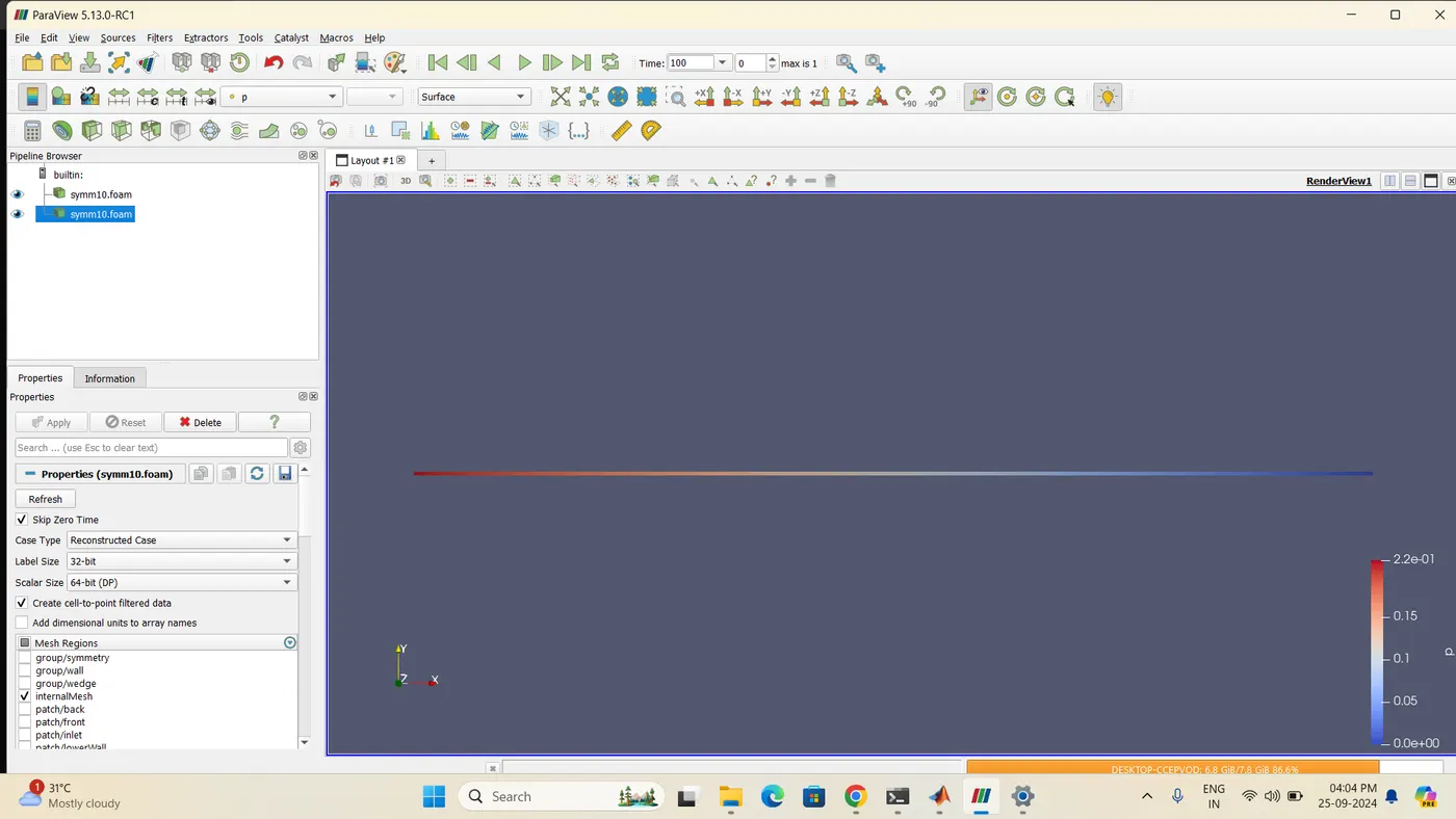
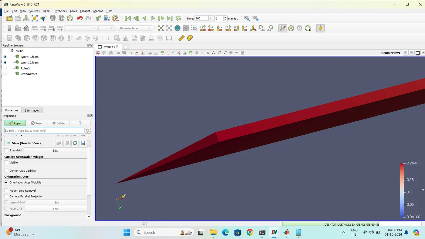
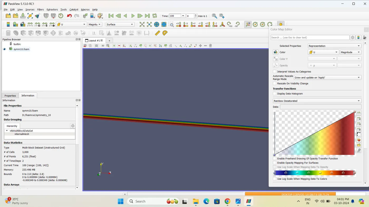
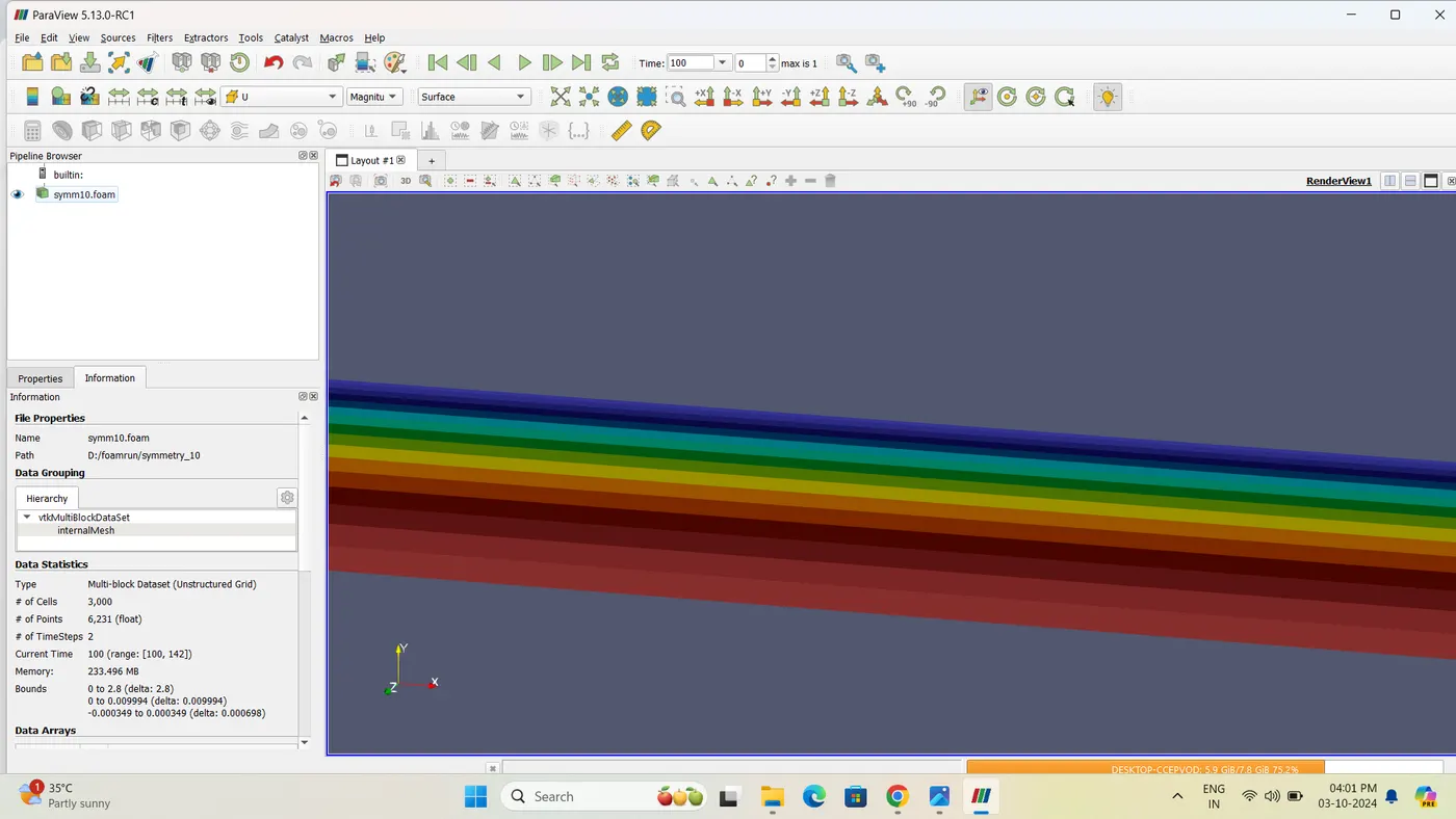
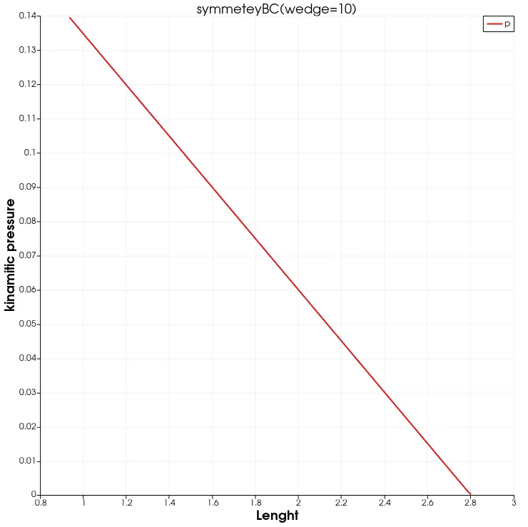
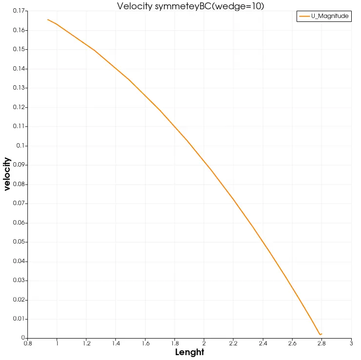
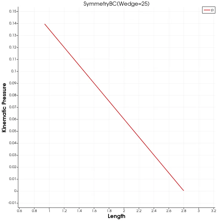
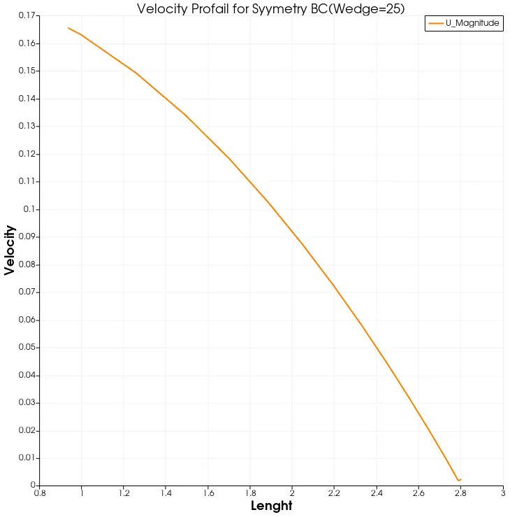
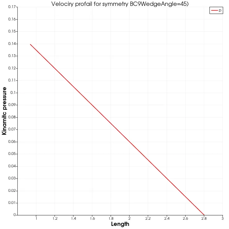
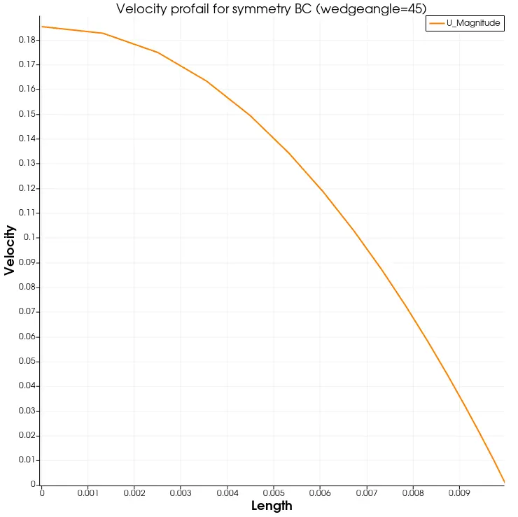
Results and Graphs different Angeles 10,25,45 :-

Hagen_Poiseuille's Thery:-

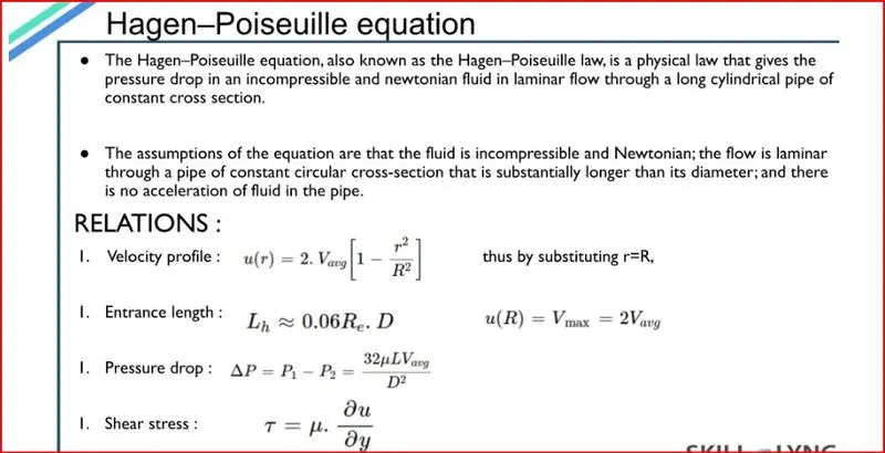
In nonideal fluid dynamics ,the Hagen-Poiseuille equation ,also known as the hagen-poiseulle law,Poiseullelaw or Poiseuille equation, is phusical law that gives the pressure drop in an in-compressible and Newtonian fluid in laminar flow flowing through a long cylindrical pipe of constant ceoss section.

The assumptions of the equation are the fluid is incompressible and Newtonian; the flow is laminar through a pipe of constant circular cross-section that is substantially longer than is diameter; and there is no acceleration of fluid in the pipe.

The pressure drop in incompressible and newtonian fluid in laminar flow through a long cylinder pipe of constant cross-section can be derived sa

The assumptions of the equation are that the fluid is incompressible and Newtonian; the flow is laminar through a pipe of constant circular cross-section that is substantially longer than its diameter; and there is no acceleration of fluid in the pipe.

The pressure drop in an incompressible and Newtonian fluid in laminar flow through a long cylindrical pipe of constant cross – section can be derived as,

p = 8mue VLR^2= 32 mueVLD^2

Where, p= pressuer Difference Between the two ends(p1-p2)

L =length of pipe

meu = Dynamic viscosity

V = velocity of Fluid

R =pipe radius

D = pipe Diameter.

The ratio of length to radius of a pipe should be greater than one forty-eighth of the Reynolds number for the Hagen–Poiseuille law to be valid. If the pipe is too short, the Hagen–Poiseuille equation may result in unphysically high flow rates.

A few examples in which the Hagen–Poiseuille law is practically applied is the air flow in lung alveoli, or the flow through a drinking straw or through a hypodermic needle. It is also applied for the process of blood flow through a narrow constriction.

p= 8mue*v*l/r^2 =32mue*VL/D^2 p= 8mue*v*l/r^2 =32mue*VL/D^2

Where,

PΔp${\displaystyle \Delta p}$Re =2100 Pressure difference between the two ends(p1-p2)5D

LD=0.02 Length of the pip

mue M = Dynamic V = Velocity of Fluid

V = Velocity of Fluid

D2= 0.01 pipe radius

DM = pipe Diameter

The ratio of length to radius of a pipe should be greater than one forty-eighth of the Reynolds number for the Hagen–Poiseuille law to be valid. If the pipe is too short, the Hagen–Poiseuille equation may result in unphysically high flow rates.

A few examples in which the Hagen–Poiseuille law is practically applied is the air flow in lung alveoli, or the flow through a drinking straw or through a hypodermic needle. It is also applied for the process of blood flow through a narrow constriction.

Equations and Calculations:-

We are considering the working fluid flowing inside the cross section of the pipe to be Air at an ambient temperature of

Given Data :-

Geometry of the flow is axi - symmetric.The flow is laminar and flows through a constant cross section.

1. The flow is laminar and flows through a constant cross section.
   
   
2. Inlet Reynold’s Number, Re= 2100reo=997.

Wedge angle should be less than 5Dkgm^3

Analytical solution ameter of the pipe

:- CONCLUSIONS:

From the above study,we have successfully simulated an axi-symmetric flow by applying the wedge boundary condition across aconstant criss section pipe ,for an inlet Reynold's of 2100 and a wedgr angle of 4*

:-The Matlab code to automate the generation of of the block Mesh Dict File has been successfully written ,which takes the provided inputs and outputs a fully functional blockMeshDict files as shown above.

:-From the simulation run we obtain our respective

From the simulation run, we obtain our respective and as shown above. To study the velocity profiles, we carry out a test to study the flow characteristics at different regions of the pipe. We study the velocity profile plots at of the pipe, at a distance of from the inlet of the pipe.

:- From the plots obtained, we can observe that the fluid velocity at the walls of the pipe remains , due to the we have provided. We can also observe that the velocity profiles slowly develop and become more and more sharper () as the distance from the inlet increases.From the simulation run, we obtain our respective and as shown above. To study the velocity profiles, we carry out a test to study the flow characteristics at different regions of the pipe. We study the velocity profile plots at of the pipe, at a distance of from the inlet of the pipe.

:- from the simulation run ,We obtain our respective Wedge Geometry and velocity profiles aas show above . To study the velocity profile ,we carry out a test to study the flow characteristic and different regions of the pipe .

We study the velocity profile plots at regions of t he pipe,Distance of 2.8m(outlet) from the inlet of the pipe.

:- from the plots outlined,We can observe that the fluid velocity at the walls of the pipe remains Zero,due to the no_slip boundary condition we have provide .we can also observe that velocity profiles slowly develop and decome and more sharper (parabolic) as the distance from the inlet increases.of the pipe ,which is referred to as the of pipe

:- Due to the no -slip conditions at the walls of the pipe ,the abjacent of the fluid tend to slow down as the flow progresses,due to friction created between these layers .This leads to an increase in velocity of the at the centre of the pipe As a result ,the velocity profiles keep developing as the distance from the inlet increasea and the fluid reaches Mamximum velocity at the outlet of the pipe ,which is refrred to as the fully developed region

:- From the pressure plots obtained from the simulation, we can observe that the fluid pressure is the highest at the inlet of the pipe and theredy,we can say that the pressure drop obtained from this simulation obeys the Hagen-Poiseuille'sTheory.

:-Shear Stresses are developed in the fluid as a result of relative motion of the fluid layers adjacent to the walls of the pipe ,Which are provided with a no-slip boundary condition,leading to the walls of the pipe being Zero.From the shear steer's plot obtained, we can observe that the stresses are maximum at the walls of the pipe and it slowly decrease as it reaches the center of the pipe,as the relative friction between the layers slowly decrease.

:-Comparison between the Boundary Conditions.

We have performed Simulation for two Boundary Conditions,those are Symmetry Boundary Conditions and Wedge Boundry Condition.

During the wedge Boundary conditions conditions simulation,the simulation across the arc of the wedge is not done ,but whereas in the code OD Symmetry

Boundary Condition,the calculation across the are of the wedge is done, hence the simulation time is higher in that case.The Courant number and hence the Symmetry Boundary condition wil be slightly more accurate. The Symmetry Boundary conditions consider the Mesh as 3D and the calculation is done along all the three global axes.

We understand the results should not changing due to the changing in the Boundary conditions ,and this is because the Physics of the problem does not changing and remains the same

Conclusion In conclusion , I would like to start that this challenge helped me understated the difference between the two boundary conditions and how to simulation then as per the need of the problem that we will be simulating.