Week 10: Project 1 - FULL HYDRO case set up (PFI)

Simulation of Port Fuel Injection (FULL HYDRO)

Objectives: To perform a full hydro simulation on a Port Fuel Injection geometry and analyze the results.

Port Fuel Injection:

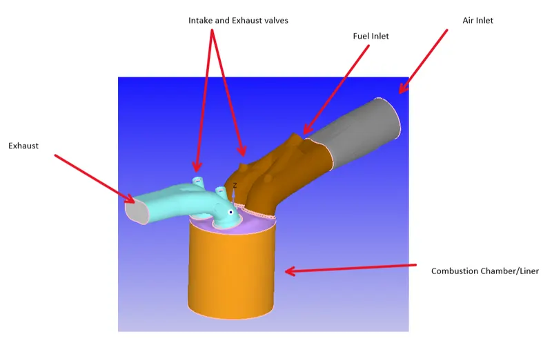
The above figure shows the Port Fuel Injection geometry of a Gasoline Engine. It consists of simplified regions such as air inlet, fuel inlet, exhaust, etc.

The geometry is divided into different regions which help to define events such as opening and closing of valves and splitting of ports helps to assign better initial conditions.

Various boundary surfaces are listed below briefly;

Piston:

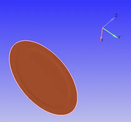
The above figure shows the piston face which reciprocates to compress the air-fuel mixture and initiate combustion.

Liner:

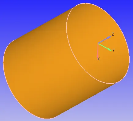
The liner geometry is the region through which the piston face reciprocates. In other terms, liner forms the basis of a combustion chamber.

Cylinder head:

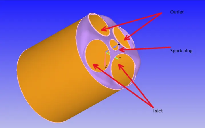
The cylinder head consists of ports such as a fuel inlet, exhaust outlet, and spark plug. They are located on top of the liner perpendicular to the reciprocating motion of the piston face.

Intake and exhaust valves:

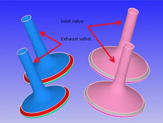
Inlet and exhaust valves facilitate the intake of air-fuel mixture and expel exhaust emissions. They work based on a timing cycle. When the piston moves to the BDC, the inlet valves open, and when the piston moves to TDC initiates combustion thereby exhaust valves open to push out emissions.

Spark plug terminal:

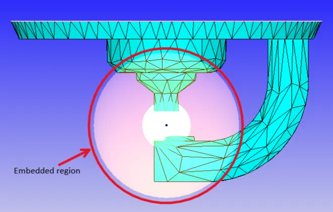
The above figure shows the embedded region around the spark plug terminal. The embedded region is formed in order to model the spark accurately which initiates combustion when the air-fuel mixture comes into contact. Further details of embedding levels are discussed in this report at a later stage.

Intake region:

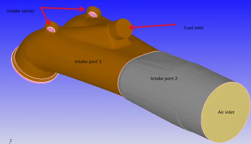
Two different regions intake ports 1 and 2 are defined separately in order to assign initial conditions separately. Fuel inlet and air inlet and located at different points with different sizes.

Exhaust/Outlet region:

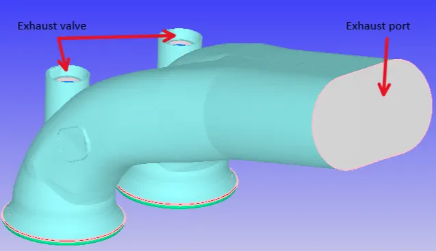
Similar to inlet regions facilitating the flow of air-fuel mixture, the exhaust port facilitates the removal of emissions post-combustion.

Materials:

Gas Simulation: ON (Temperature dependent)

Species/Parcels: IC8H18, Mol. weight 114.231 kg/kmole, Critical Temperature 543.8

Engine Geometric Parameters:

1. Bore =0.086 m
2. Stroke = 0.09 m
3. Connecting rod length = 0.18 m
4. RPM = 3000

Run parameters:

1. Simulation mode: No Hydro
2. Turbulence Modelling: RNG k-epsilon
3. Start time: -520 deg
4. End time: 120 deg

Boundary conditions:

1. Piston temperature - 450K
2. Liner temperature - 450K
3. Head temperature - 450K
4. Spark Plug temperature - 550K
5. Spark Plug electrode temperature - 600K
6. Exhaust ports temperature - 500K
7. Exhaust outflow - 1 bar
8. Exhaust outflow temperature - 800k
9. Exhaust species concentration - Calculate the stoichiometric condition
10. Exhaust valve top temperature - 525K
11. Exhaust valve angle temperature - 525K
12. Exhaust valve bottom temperature - 525K
13. Intake port - 1 temperature 425K
14. Intake port - 2 temperature 425K
15. Inflow pressure - 1 bar total pressure
16. Inflow temperature - 363K
17. Inflow species - Air
18. Intake valve top temperature - 480K
19. Intake valve angle temperature - 480K
20. Intake valve bottom temeprature - 480K

Initial conditions:

• Intake port - 1 (closer to combustion chamber)
  • ic8h18 - 0.025508
  • o2 - 0.20157
  • n2 - 0.77292
  • Temperature - 390k
  • pressure - 1 bar
• Intake port - 2 (away from combustion chamber)
  • Air
  • Temperature - 370K
  • Pressure - 1 bar
• Cylinder
  • Pressure - 1.85731 bar
  • Temperature - 1360K
  • Stoichiometric composition

Injection Parameters:

1. Fuel flow rate = 7.5e-4 Kg/second
2. Injection start time = -480.0
3. Injection duration = 191.2
4. Fuel temperature = 330K

Nozzle positions:

Nozzle diameter = 250 micro-meter

Circular injection radius = Nozzle radius

Spray cone angle = 10

• Nozzle 0
  • center 0.0823357 0.00100001 0.07019
  • Align Vector -0.732501 0.210489 -0.647408
• Nozzle 1
  • center 0.0823357 -0.00099999 0.07019
  • Align Vector -0.732501 -0.210489 -0.647408
• Nozzle 2
  • center 0.0823357 -0.0004 0.07019
  • Align Vector -0.5 -0.2 -0.647408
• Nozzle 3
  • center 0.0823357 0.0003 0.07019
  • Align Vector -0.5 0.2 -0.647408

Events:

Events are assigned to perform certain actions such as movement of boundary (eg. rupture of diaphragm, reciprocating of the piston, valves, etc at a specific time period.)

The above event is cyclic which is assigned to Intake and Exhaust valve movements at specified Crank angles.

Intake ports 1 and 2 facilitating intake of air and fuel is set to a permanent event as open.

Spray Modeling:

Converge uses Eulerian solver to solve gaseous sprays and Lagrangian solver to solve liquid sprays.

The concept of parcels is used in converge. A parcel is a collection of drops having the same radius, velocity, temperature, etc. Equations are solved on a per parcel basis rather than a per drop basis as the properties of drop inside the parcel are identical.

These parcels undergo several physical processes such as

• Primary breakup
• Secondary breakup
• Drop drag
• Collision and Coalescence
• Turbulent dispersion
• Evaporation

The below figure shows various physical processes during spray breakup.

Spray Modeling setup:

General - Drop Evaporation:

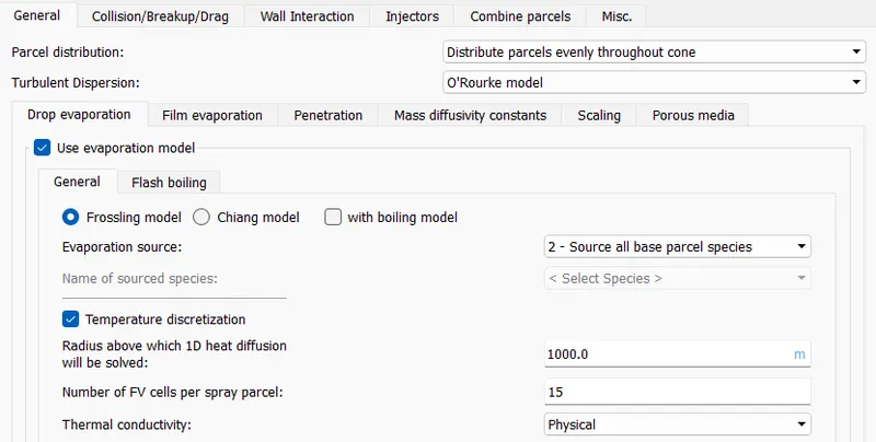
• In the above section, parcel distribution is specified to be evenly distributed through the cone. There is another option that would distribute parcels evenly along the axis of the cone.
• Turbulent dispersion is enabled using the O'Rourke model which is an LES-based Turbulent kinetic energy preserving model. Turbulent dispersion is a phenomenon that the spray parcels undergo due to fluctuations of turbulence.
• The evaporation model is enabled using the Frossling model which computes at what rate does the drop evaporates.
• The evaporation source is set to source all base parcel species. There is also an option to source specified species that evaporates to specific species and also to source into all-composite parcel species which will aid in the case of multi-component liquid species.
• Temperature-based discretization is turned on with 1000m as the threshold radius of a parcel above which the 1D heat diffusion equation will be solved. If the drop radius exceeds the max value (here, 1000m), converge will assume a radially varying temperature distribution else it will assume a uniform temperature distribution.

General - Film Evaporation: OFF

General - Spray penetration:

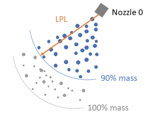
• Spray penetration length is calculated using the mass fraction. Here, 0.95 of the mass fraction is set as the threshold for estimating spray penetration which means that first the total mass of the liquid parcel is calculated from the nozzle and then this mass is multiplied by the liquid penetration fraction to yield the penetrated spray mass. Starting from the center of the nozzle hole, CONVERGE sums up the mass of the liquid parcels until it reaches the penetrated spray mass. This distance is the LPL.

• For calculating Vapor penetration length, two parameters are considered. (a) Fuel vapor mass fraction exceeds the user-specified fuel vapor mass fraction. (b) The cell size does not exceed the user-specified bin size. It is recommended to have a bin size at least twice the size of the cells in the spray cone. Here, the bin size is set to 0.001m, and the minimum fuel vapor mass for considering into VPL calculation is 0.001. The below figure illustrates the calculation of VPL.

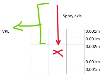
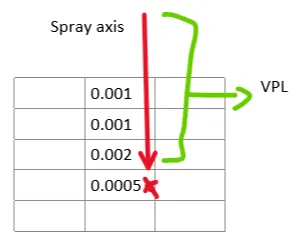
Fig. Cell size condition (a-Left), Fuel vapor mass fraction (b-right)

General - Mass diffusivity constants: Set as defaults for n-Tetradecane as the properties are close to default species.

General - Scaling: All set to 1 (zero scaling)

General - Porous Media: OFF

Collision/Breakup/Drag:

Whenever two spray drops come into contact with each other, they pass through or breakup, or coalesce. Such phenomena are modeled under this section.

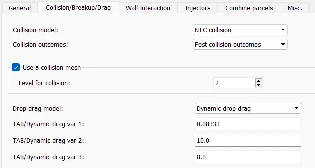
• The collision of spray drops is modeled using NTC collision and post-collision outcomes are chosen.
• The collision mesh is turned on. It creates a separate adaptive collision mesh which reduces grid sensitivity when two parcels collide in the same cell. Turning this on enables the collision of parcels across grid cells.
• Drop Drag is the drag effect experienced by a drop. Converge provides options to eliminate drag consideration using the No Drag Drop model, to assume the drops are perfect sphere, to account for variations in drop shape which brings in a TAB model to determine distortion.

Wall Interaction: Wall film

Available interactions are Rebound/Slide after impingement, Wall film approach where drop actions are calculated with a hybrid approach based on particle/film based quantities, vanishing of drop after interaction which is not advisable as it leads to mass loss.

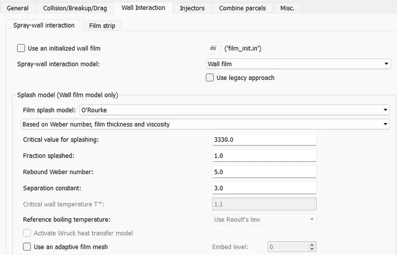
Wall film model is set to O'Rourke which models splash criteria based on Weber number and film thickness.

Combustion Modeling Setup:

• Converge offers two types of solvers such as SAGE (detailed) and simplified models for combustion modeling. SAGE model is accurate but slow whereas the simplified model works in an opposite manner. SAGE uses local conditions in each cell to calculate reaction rates based on the principle of chemical kinetics.

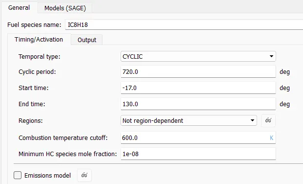
• Fuel species are set to IC8H18 which resembles properties similar to petrol. Start and End time in terms of degrees are defined with sequential cycle time.

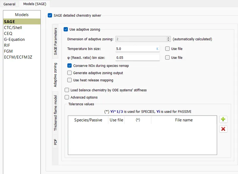
• Multi-zone model (adaptive zoning) is enabled which is a technique in CONVERGE that reduces the number of SAGE calculations by grouping cells into bins. A number of bins vary dynamically with the stratification of flow field parameters. Bins are created based on two or more variables such as Equivalence ratio, Temp, Pressure etc.
• This technique enables calculation of average quantities and SAGE solver solves once per bin instead of each cell.
• Conserve NOx is enabled to remap species after solving which improves N2 prediction.

Source/Sink Modelling:

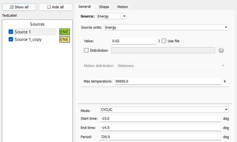
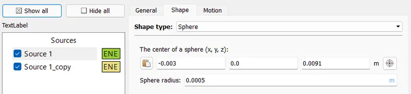
Two levels of a source are applied at the spark plug region with a temperature of 50000K using a uniform sphere shape.

Grid Generation:

A baseline grid of 0.004m along all 3 directions is generated.

Adaptive Mesh Refinement:

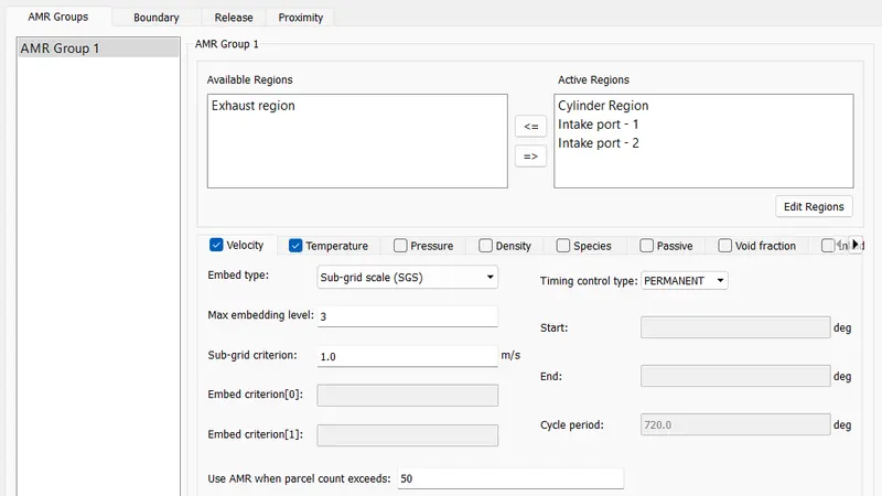
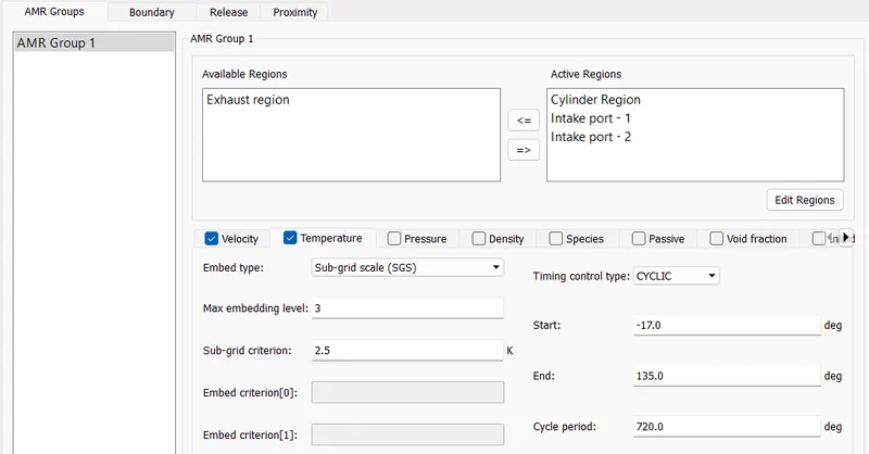
• A velocity and temperature-based AMR is applied with a Sub-grid scale embedding level of 3 and a criterion is set to be 2.5K difference with respect to temperature curvature () and 1m/s with respect to velocity.
• Velocity-based AMR is applied permanently whereas Temperature based AMR is applied for a specific crank angle period.

• The refined grid size is given by the above expression (i.e., 0.004/2^3 =0.0005m)

Fixed Embedding:

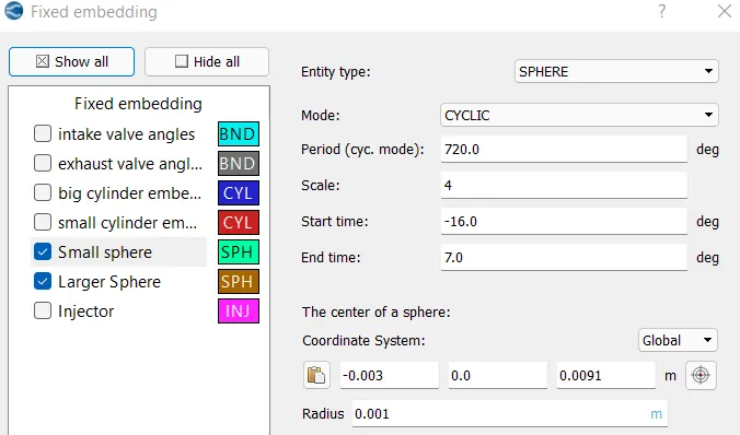
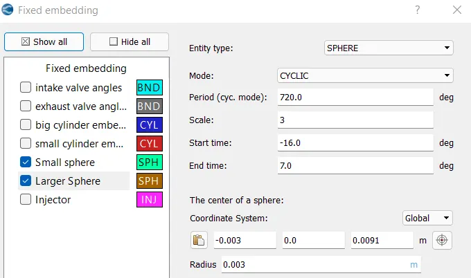
Fixed embedding refines the grid along the boundary without any conditions, unlike AMR. In the above snapshots, it is evident that two layers of embedding are applied to scale down the mesh by a factor of 3 and 4 at two circumference levels.

A sectional view of grid generation:

Results/Inferences:

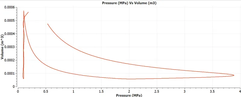
PV diagram:

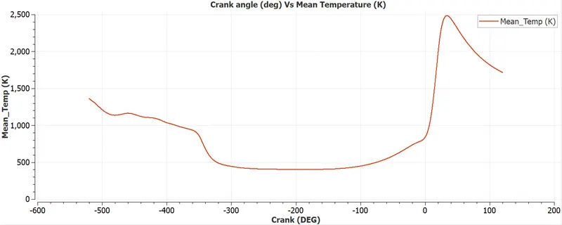
Mean Temperature:

Compression ratio:

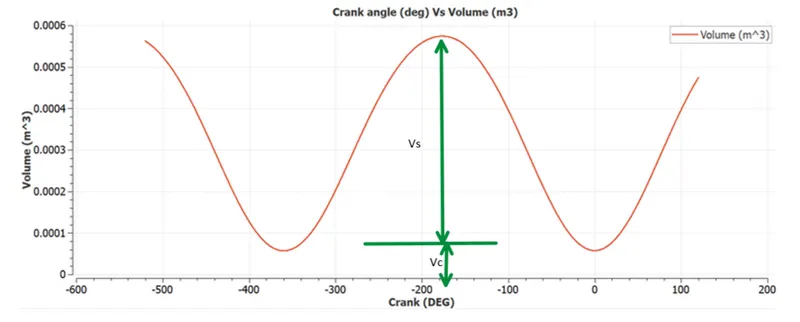
Stroke Volume:

Clearance Volume:

Compression ratio = Total Volume/Clearance Volume = (Vs+Vc)/Vc

Here, Vs - Swept Volume, Vc - Clearance Volume

CR = 11.06

Wall heat transfer model:

• Heat transfer occurs through conduction, convection, and radiation. CFD governing equations solve mass, momentum, and energy equations related to compressible/incompressible fluids.
• The energy equation in NS equations can predict the temperature distribution across the fluid domain using a source term. However, to model a heat transfer through the wall, a separate set of equations are required to predict the heat transfer through the solid such as conduction.
• For this purpose, Conjugate heat transfer techniques are used. Converge uses a solid heat equation coupled with a CFD solver to estimate accurate wall heat transfer.
• If only a CFD solver is used, the temperature near the wall can be estimated but not the exact heat transfer across surfaces.

Combustion efficiency:

The combustion efficiency η_c is defined as the ratio between the energy released by the burnt fuel and the theoretical energy content of the fuel mass during one complete engine cycle.

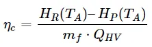
where;

H_R [J] – enthalpy (internal energy) of the reactant
H_P [J] – enthalpy (internal energy) of the product

Hr-Hp = total energy released after combustion
T_A [K] – ambient temperature
m_f [kg] – the mass of fuel inducted per cycle
Q_HV [J/kg] – the heating value of the fuel,

The heating value (also known as energy value or calorific value) of a fixed quantity of fuel, is the amount of heat released during its combustion. The heating value of a fuel is the magnitude of the heat of reaction measured at constant pressure/volume and standard temperature (26 °C) for the complete combustion of a unit of mass of fuel.

Any fuel has two types of heating values:

• higher heating value (HHV), also known as gross heating values
• lower heating value (LHV), also known as net heating value (is determined by subtracting the heat of vaporization of the water from the higher heating value)

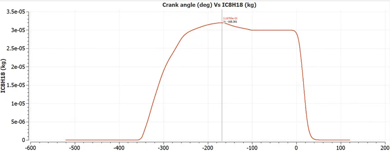
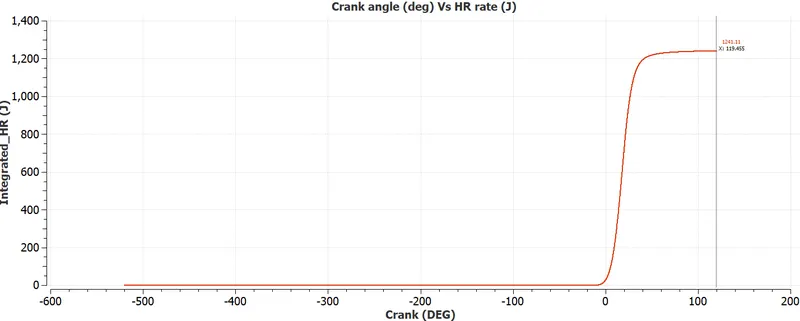
From the above two plots following observations are made;

Mass of fuel per cycle= 3.197e-5 kg

Heat release = 1241.11 J

Higher heating value of octane = 44.427 MJ/kg = 44427 KJ/kg

ηc = 87.3%

Volumetric Efficiency:

The volumetric efficiency η_v is defined as the ratio between the actual (measured) volume of intake air V_a [m³] drawn into the cylinder/engine and the theoretical volume of the engine/cylinder Vt [m³], during the intake engine cycle.

η_v = V_a / Vt

The volumetric efficiency can be regarded also as the efficiency of the internal combustion engine to fill the cylinders with intake air. The higher the volumetric efficiency the higher the volume of intake air in the engine.

In the case of indirect fuel injection engines (mainly gasoline), the intake air is mixed with fuel. Since the amount of fuel is relatively small (ratio 1:14.7), compared with the amount of air, we can neglect the fuel mass for volumetric efficiency calculation.

Vt = 0.00052269381 (theoretical Vs)+ 0.000057029438 (Vc from plot) m3 = 0.000579723248 m3

Va is calculated using the ideal gas law equation.

PVa=mRT

Here, P= 1atm=101325 N/m2

R = ideal gas constant = 287

T=Temperture at STP = 298.15K

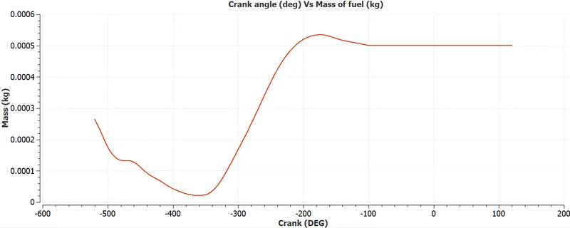
From the above plot, mass of air in kg can be 0.000534 approx (excluding fuel particles).

Therefore Va= 0.00045 m3

η_v = V_a / Vt = 77.78%

Power and Torque:

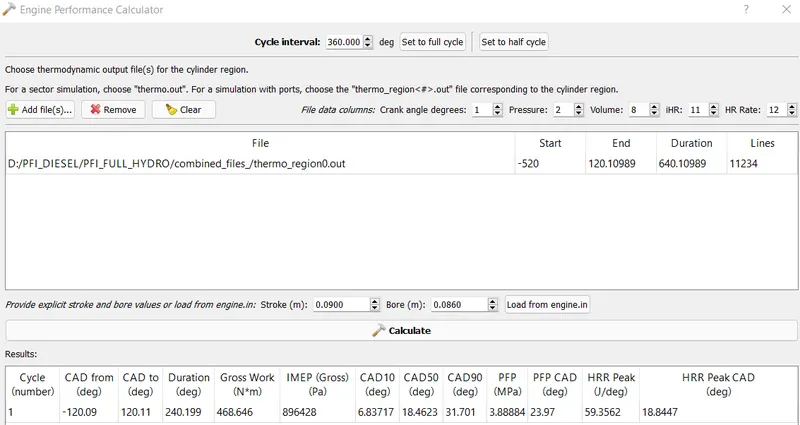
• Work = 468.646 Nm
• Duration = 240.199 deg
• RPM = 3000, RPS=3000/60=50
• Total angular rotation per second = 50*360deg=18000 deg
• Combustion Duration in seconds = 240.199/18000=0.01335 seconds
• Power = Work/Time = 468.646/0.01335 = 35104.56 J
• Torque = (Power * 60)/(2*pi*N)=111.76 Nm

Significance of CAD10, CAD50, and CAD90:

• CAD10 corresponds to the Crank Angle Degree at which 10% mass fraction burned, here 6.83 deg, signifies the ignition delay/lag.
• CAD50 corresponds to the Crank Angle Degree at which 50% mass fraction burned, here 18.46 deg, signifies the end of premixed combustion or change in phase of fuel species
• CAD90 corresponds to the Crank Angle Degree at which 90% mass fraction burned, here 31.70 deg, signifies the near end of combustion.

Air mass flow rate into engine per second:

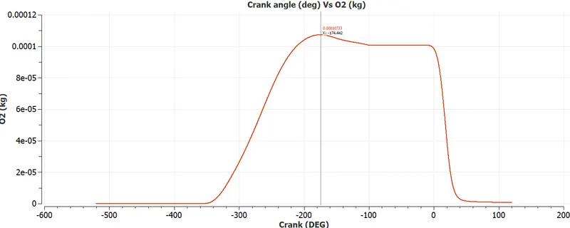
The maximum air quantity of 0.00010733kg occurs at CAD -174.442.

• RPM = 3000, RPS=3000/60=50
• Total air mass flow rate per second = 50*0.00010733= 0.0053665 kg/s

Emissions:

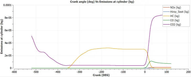
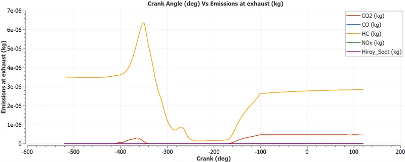
The above two plots show the emissions formed at the cylinder and emissions through the exhaust region. Emissions at the cylinder are dominated by HC which is unburnt. In general, unburnt HC is present which leads to the formation of NOx and Soot. The key factor to determine whether the engine is good or bad is by the percentage of unburnt HC. In both plots, NOx and Soot levels are minimal which indicates that the combustion is almost complete leading to a small amount of unburnt HC.

Port Fuel Injection - Spray Parcels:

Port Fuel Injection - Temperature distribution:

Port Fuel Injection - Pressure distribution:

References:

[1] Converge 3.0 Manual

[2] https://en.wikipedia.org/wiki/Heat_of_combustion

[3] https://x-engineer.org/fuel-conversion-efficiency/#:~:text=The%20combustion%20efficiency%20%CE%B7c,during%20one%20complete%20engine%20cycle.