Week 10: Project 1 - FULL HYDRO case set up (PFI)

AIM: To perform Full- hydro simulation by surface preparation and boundary flaggig using Converge CFD and post process the results using Paraview.

OBJECTIVE:

• To perform surface preparation and bounary flagging on a given IC engine case.
• Setting up Full-Hydro case setup-(PFI)simulation for the setup.
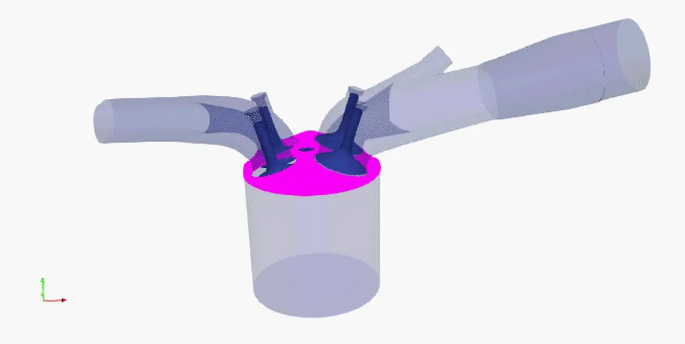
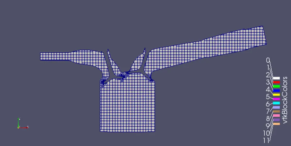
• To show the animation how all the valves and pistons move at various strokes

• Answer the following questions

  1. What is the compression ratio of this engine?

  2. Why do we need a wall heat transfer model? Why can't we predict the wall temperature from the CFD simulation?

  3. Calculate the combustion efficiency of this engine

  4. use the engine performance calculator, to determine the power and torque for this engine.

  NOTE : Since Work and Torque has the same unit (N-m) , it doesn't mean value for Torque and Work will be the same.

  Both are different quantities and has totally different meaning.

  So the value for work that you will be getting from the engine performance calculator is not the value for the torque.

  Calculate the value for the torque using the formula as shown below,

  Power(P) = (2*π*N*T)/60

  5. What is the significance of ca10, ca50 and ca90?

METHODOLOGY:

Introduction:

Port fuel injection 4 stroke model is subjected to No-hydro simulation using Converge CFD. In No hydro simulation the reactions will not be considered or Naier's stokes equations will not be solved but mesh and part movement will be checked. On confidence gained through No Hydro simualtion we proceed to Full hydro simulation. PFI involves fuel injection in the port / intake port which enters the combustion chamber through the inlet valve.

PROCEDURE:

1. Geometry

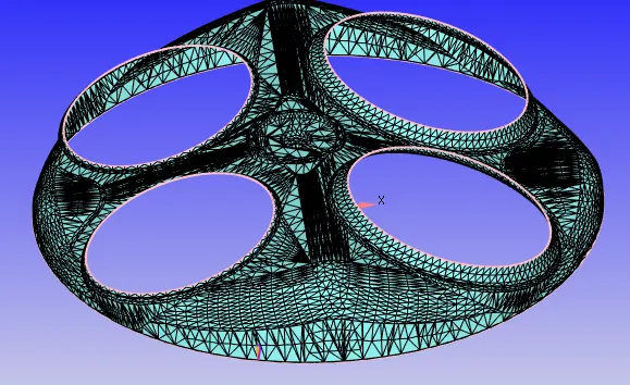
PFI geometry is imported as an stl file into the converge studio. This geometry has a number of errors that are fixed and followed by boundary flagging.

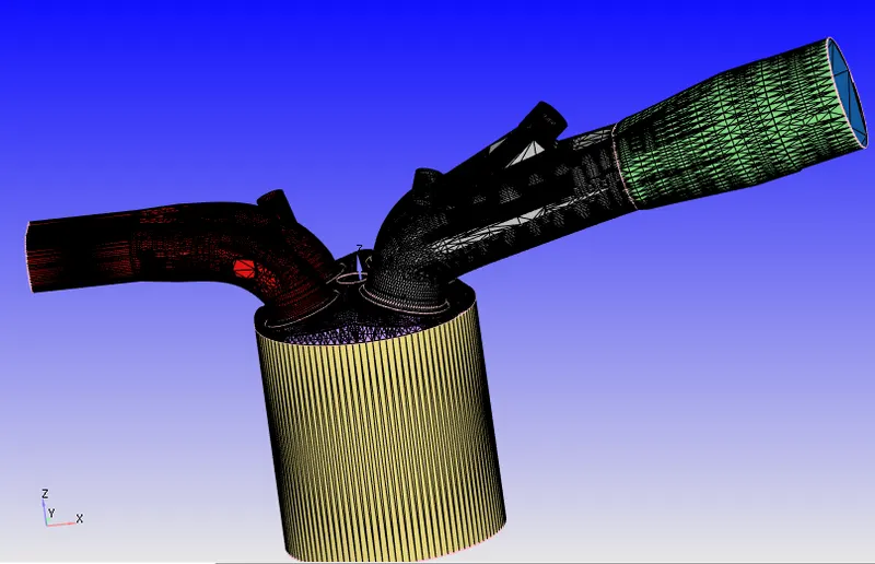
Surface Preparation and Boundary Fllaging

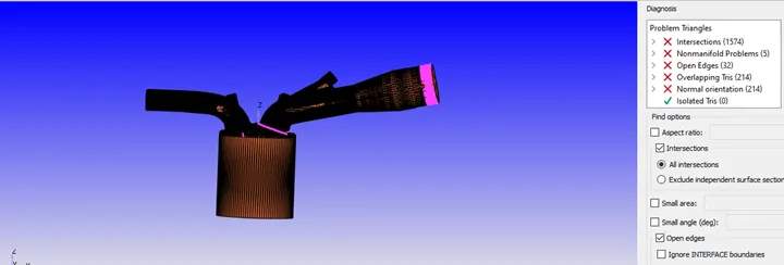
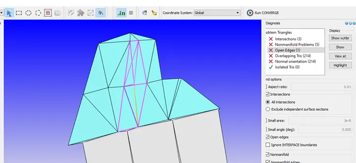
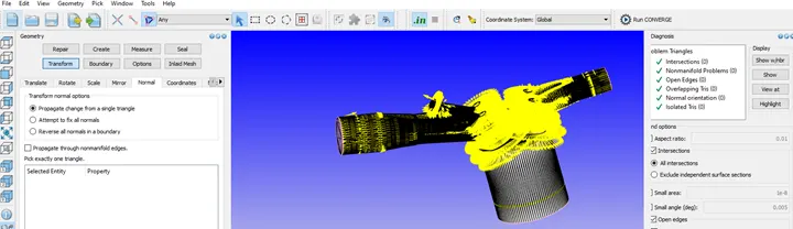
When the geometry was subjected to diagonsis intersection, nonmanifold problems. open edges and normal orientation errors were observed. Boundary Flagging aid in elliminating the errors

Boundary Flagging

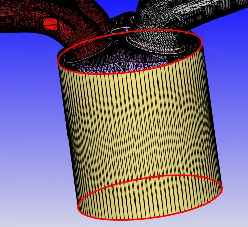
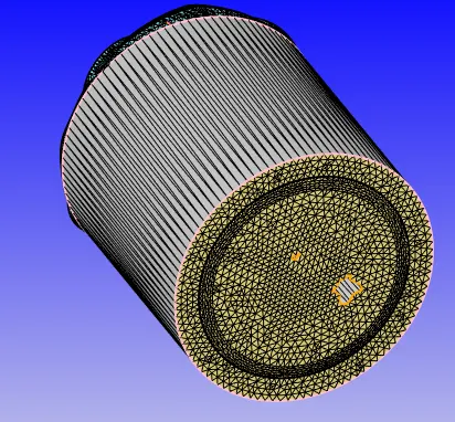
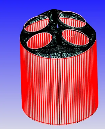
Liner and Piston

By using boundary fence and selction boundary by angle method we could flag liner and piston.

Cylinder Head

It involves removal of inlet and outlet valves for the flagging of cylinder head.

Exhaust Valve - Top, bottom and angle by bounary fence

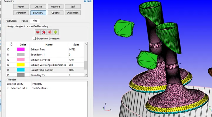
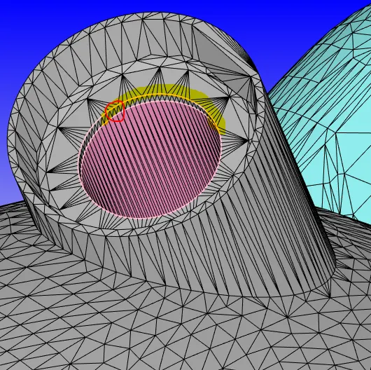
Inflow and out folow by Angle

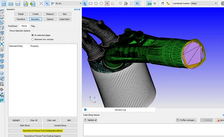
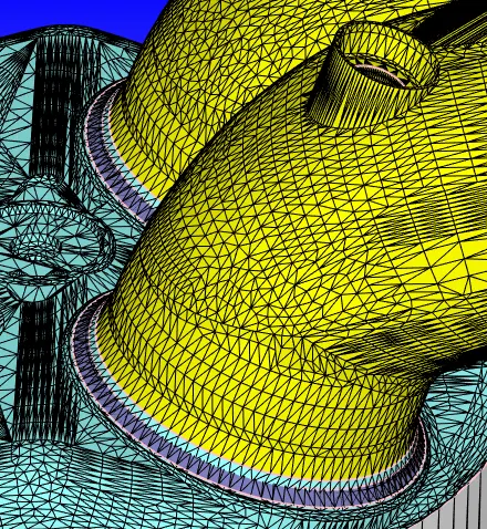
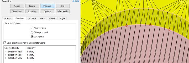
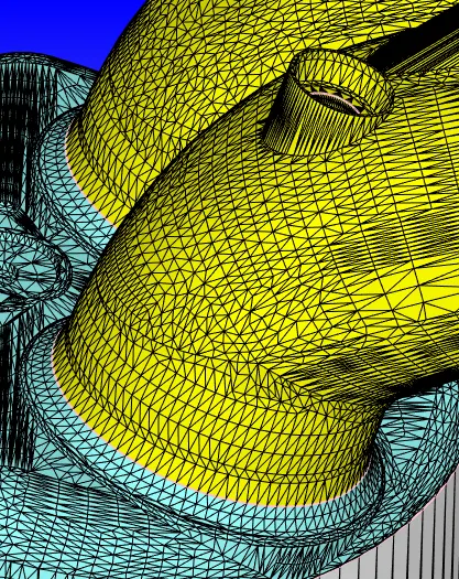
Moving Inlet valve by 0.0005 m due to interference with inlet port

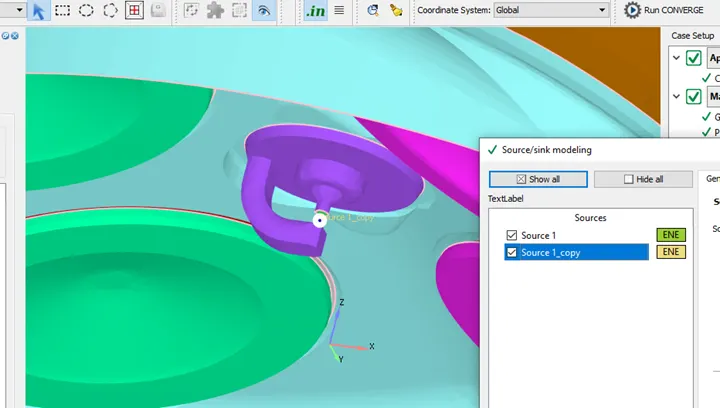
Spark Plug

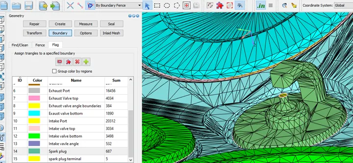
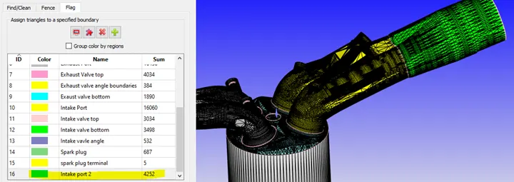
Inlet port 2 to consider the effect of parcels only in half of inlet port

Errors:

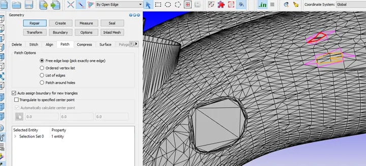
1. Open Edges

It is resolved by auto assign boundary for new triangles option under Repair Tab

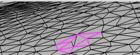
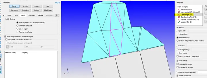
2. Intersection

One triangle is passing through the other triangle. So delete, stitch and patch them

3. Normal Orientation

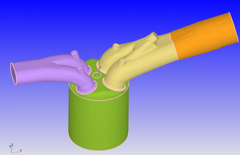
REGIONS

Case Setup-

2. Application Type

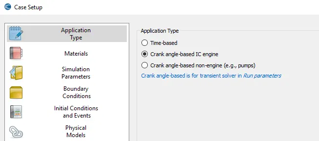
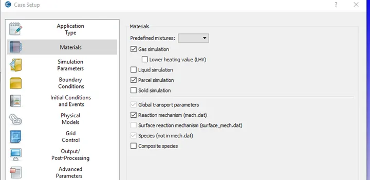
Select 'Gas Simulation' Parcel and 'species'.

Parcel in material section

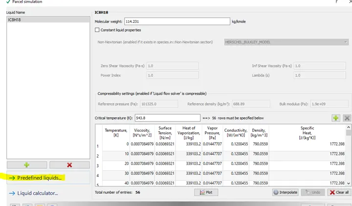
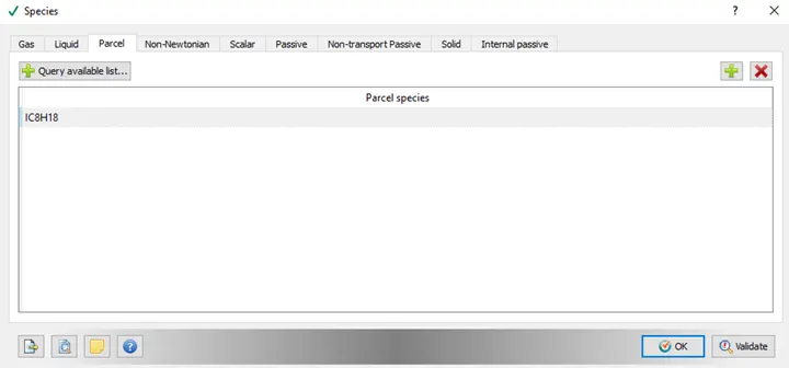
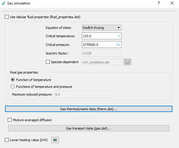
Import thermal data

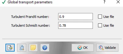
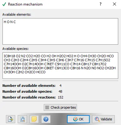
Import Mech data.

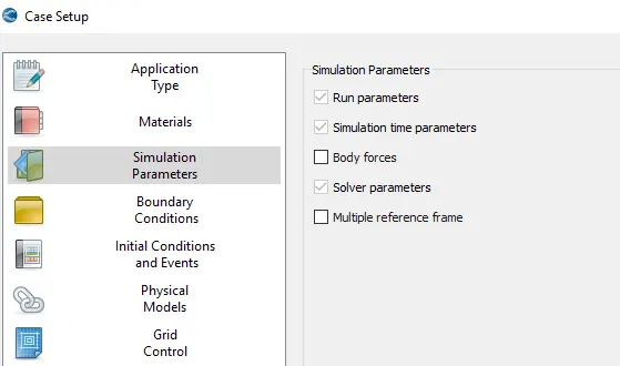
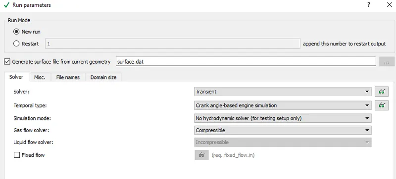
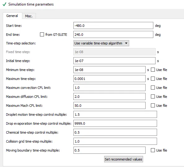
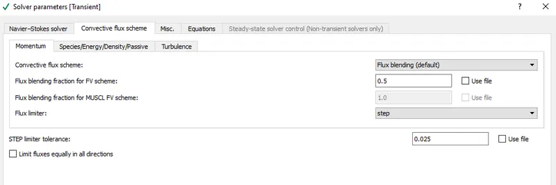
4. Simulation Parameters-

5. Boundary Conditions-

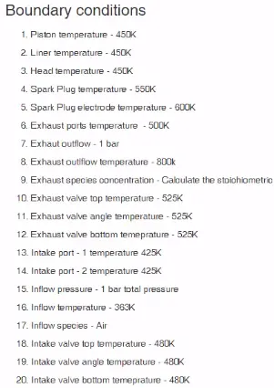
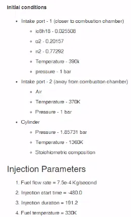
STOICHIOMETRIC EQUATION

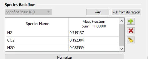
`C_8H_18 + 12.5(O_2+3.76N_2) -> 8CO_2 + 9H_2O + (3.76*12.5)N_2`

Stoichiometric Calculation
Species	MOLES	Molecular Weight (g/mol)	Mass	Mass Fraction	FORMULA
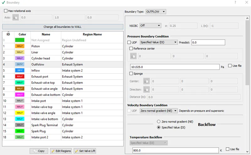
CO2	8	44.01	352.08	0.192304403	Mass fraction = induvidual mass/Total Mass
H2O	9	18.01528	162.13752	0.088558734
N2	47	28.0134	1316.6298	0.719136864	Mass =Molecular weight * Moles
		TOTAL	1830.84732	1	Total Mass = sum of Induvidual Mass

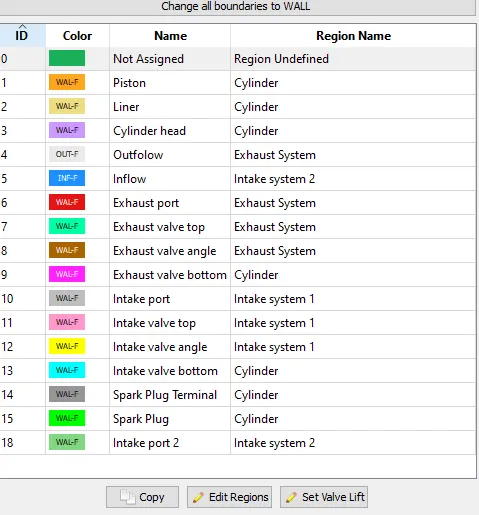
Piston:

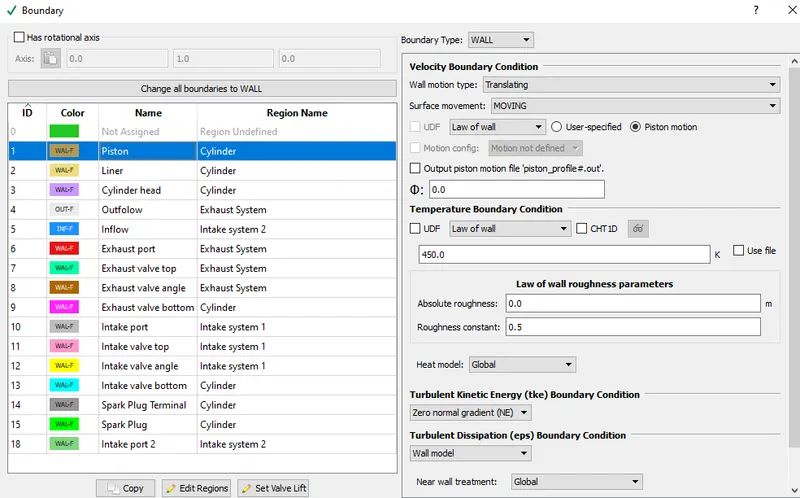
Liner

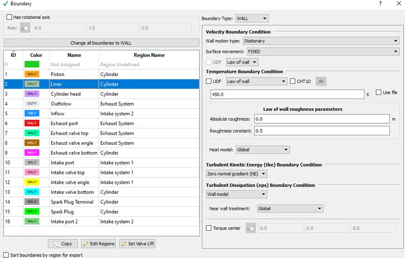
Cylinder Head

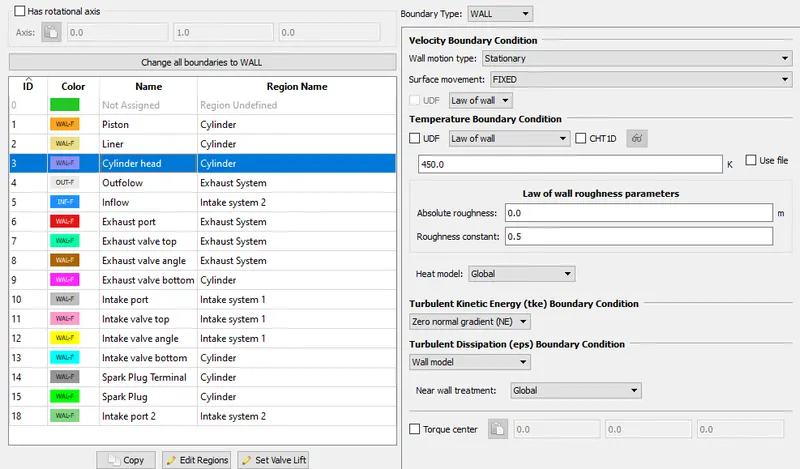
OUTFLOW

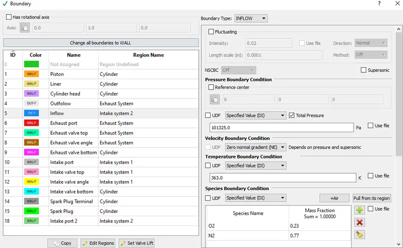
INFLOW

EXHAUST PORT

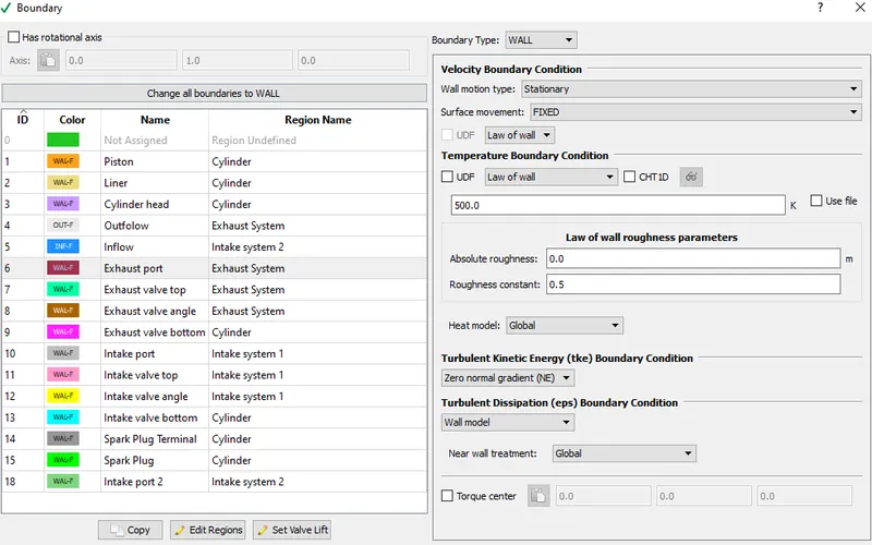
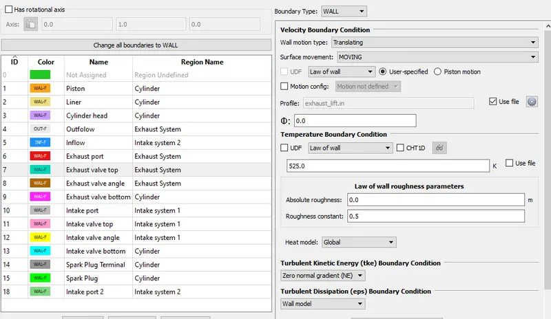
Exhaust Valve - top, bottom and angle

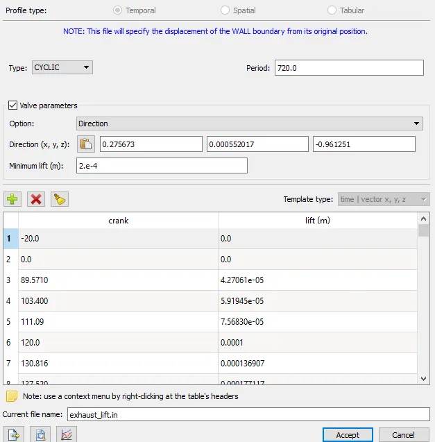
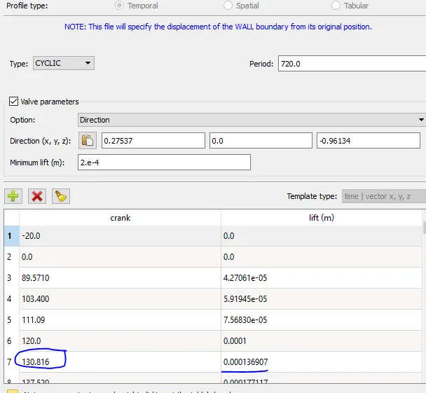
Import valve lift data and minimum lift 2 e-4 m

Intake Port

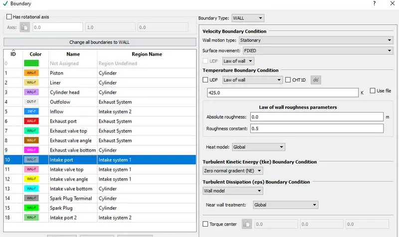
Intake Port 2

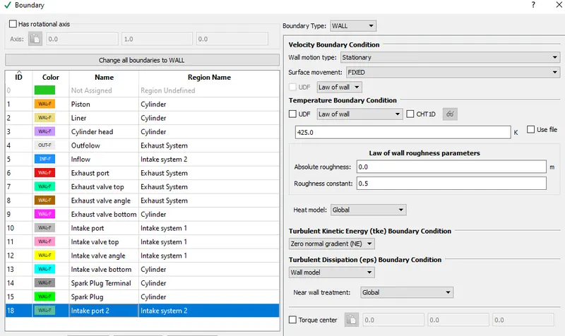
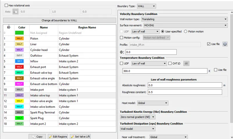
Inlet Valve - top, bottom and angle

Import valve lift data and minimum lift 2 e-4 m

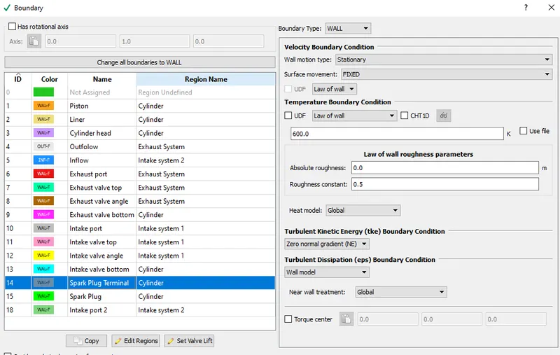
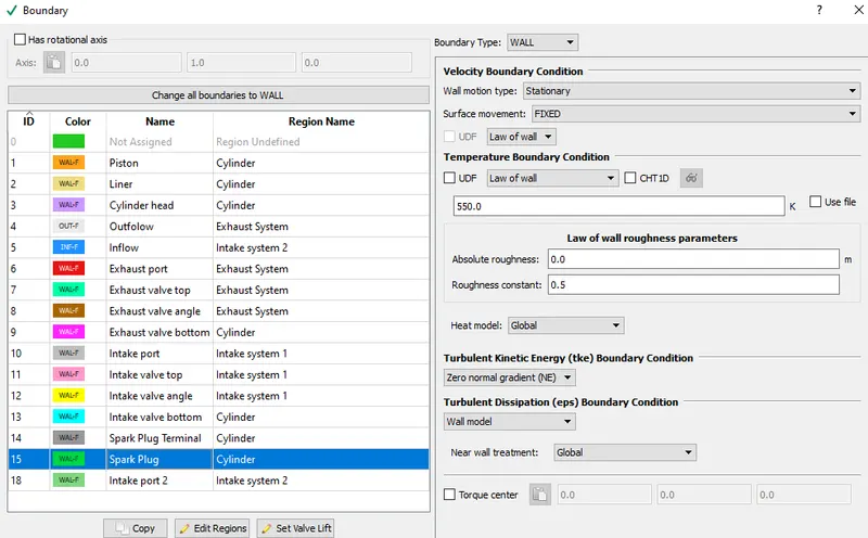
Spark Plug and Terminal

6. Initial Conditions and Events:

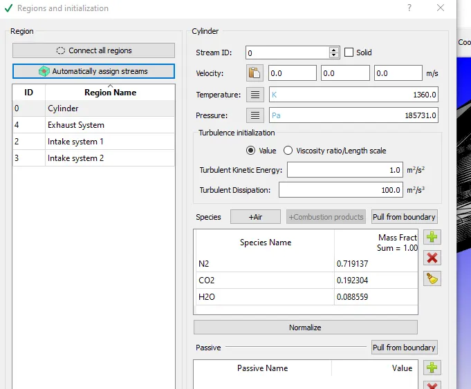
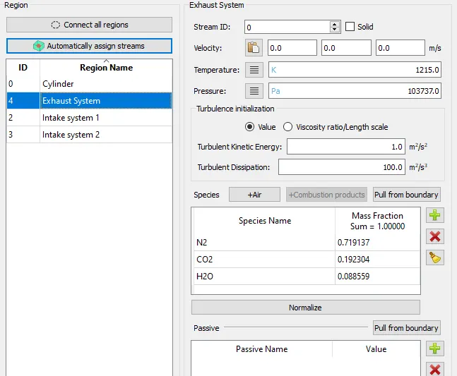
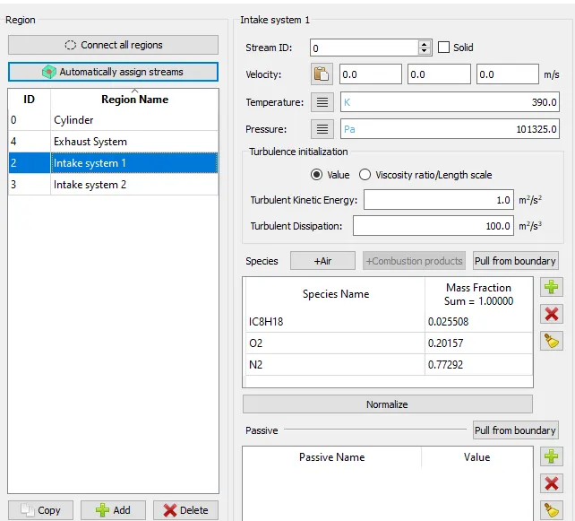
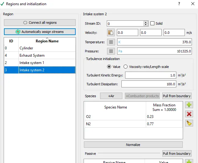
Events

7. Physical Models:

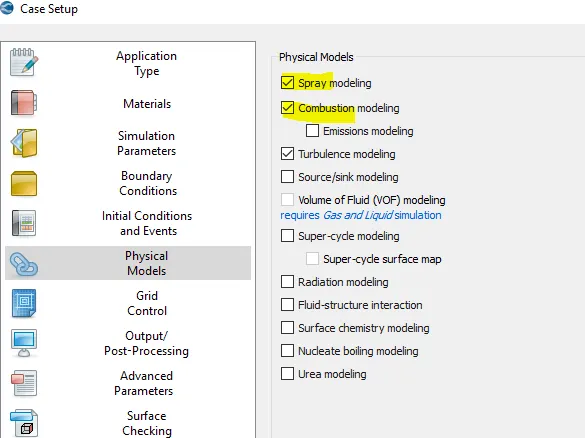
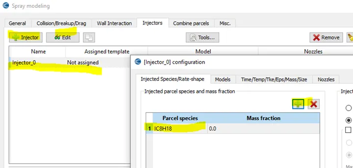
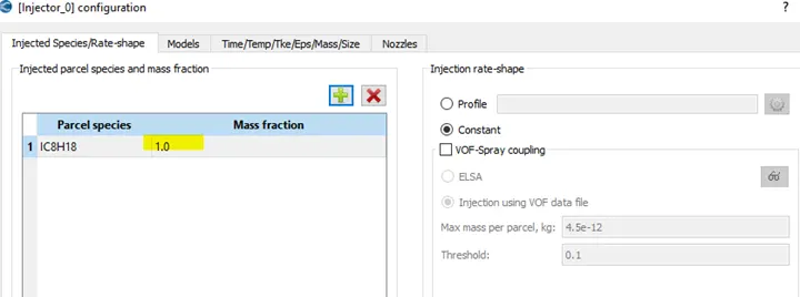
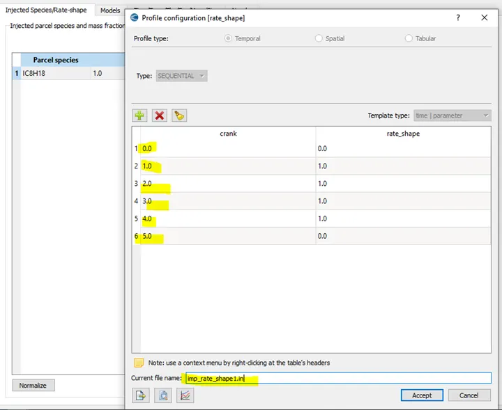
SPRAY MODELLING

Orourke model shows better performance for gasoline sprays

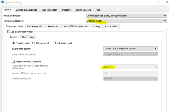
The radius here is the cut off radius below which the 1 D heat diffusion equation is not solved or temperature gradient effect in parcels below this radius will not be studied and will be considered as constant throughout the body. Small parcels we say same temp all across its body.

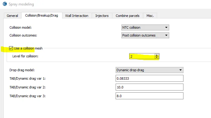
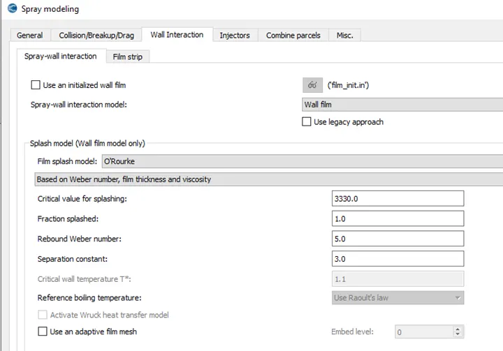
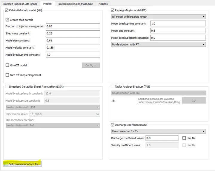
Set recommendation à Gasoline PFI

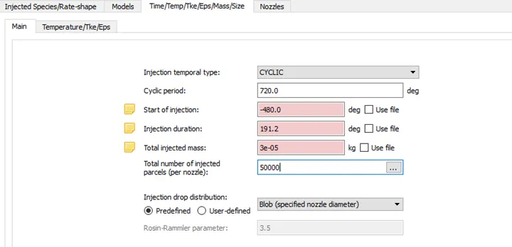
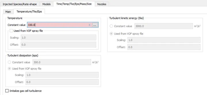
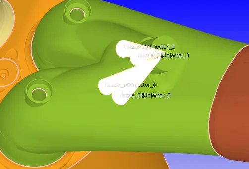
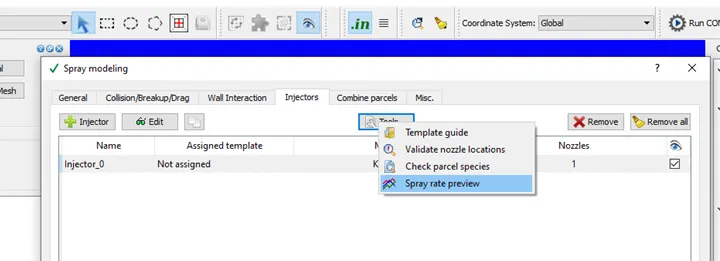
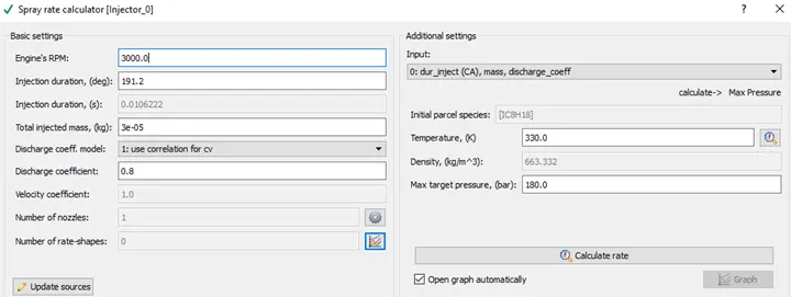
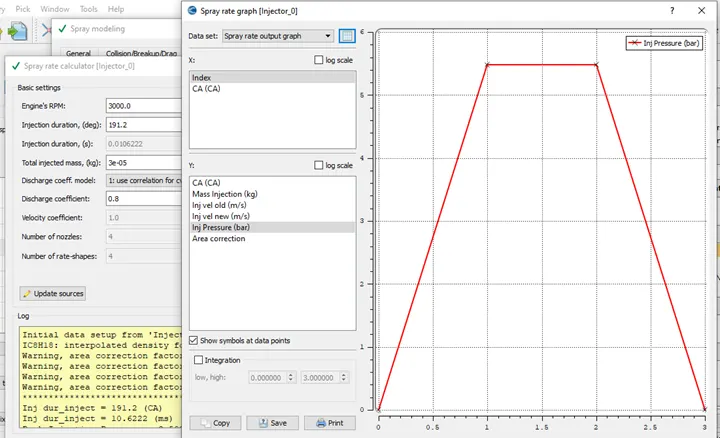
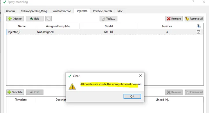
Nozzle definition

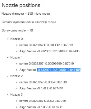
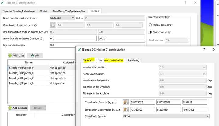
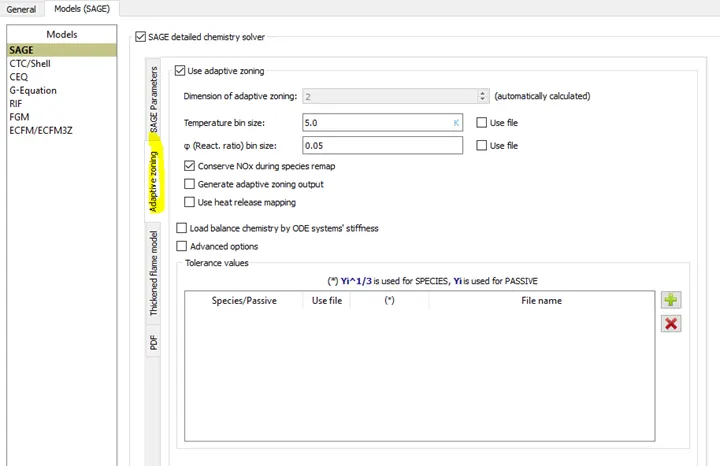
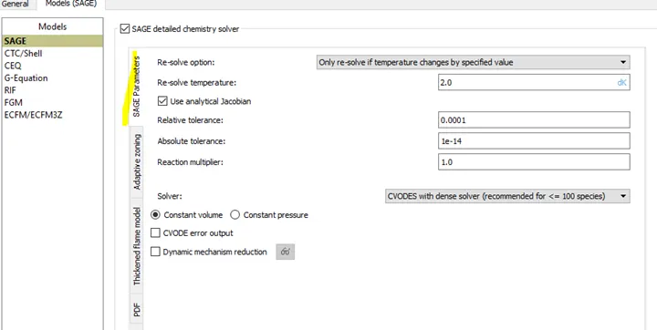
COMBUSTION MODELLING

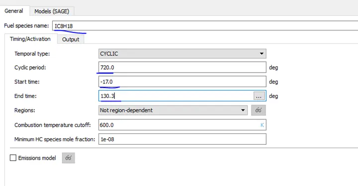
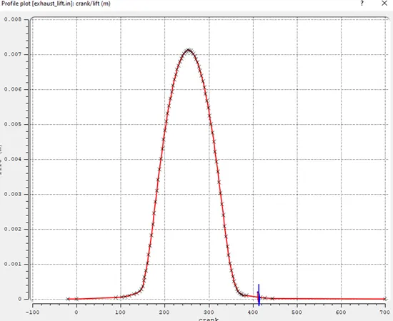
Note when exhaust valve opens – Combustion model ends or end time

When exhaust valve closes – combustion starts or start time

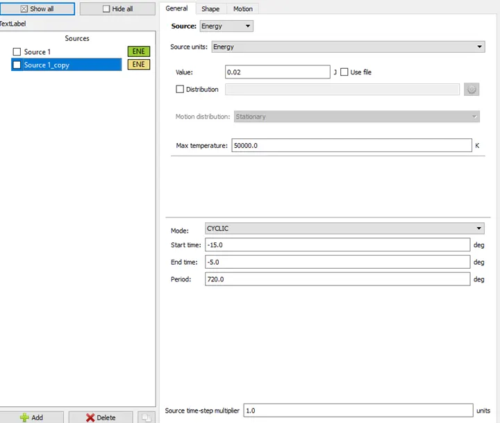
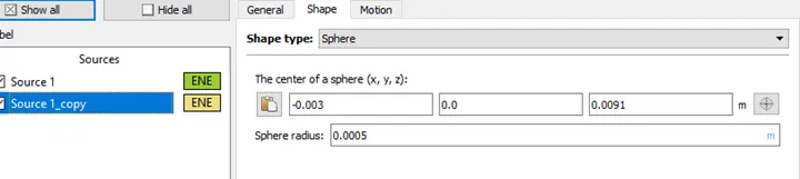
SOURCE/ SINK MODELLING

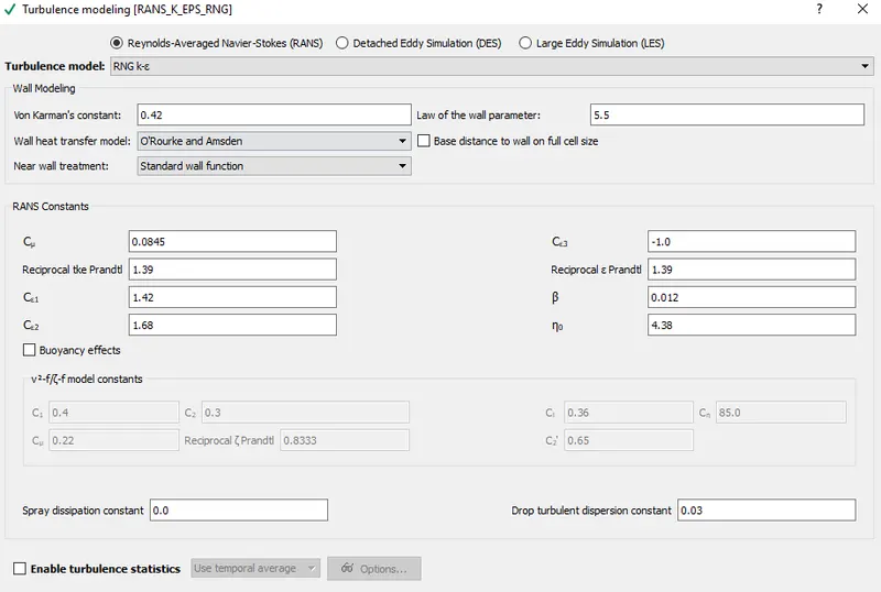
TURBULENCE MODELLING

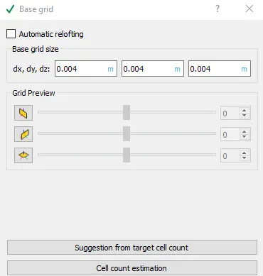
8. Grid Control:

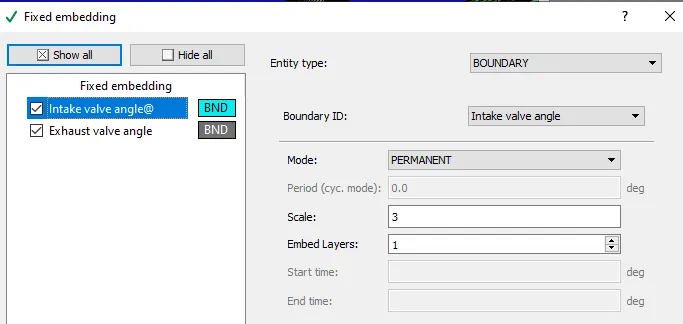
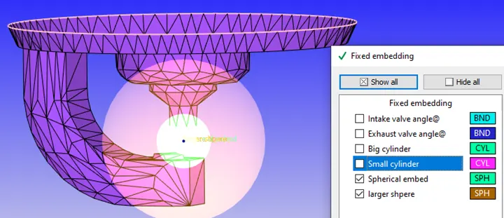
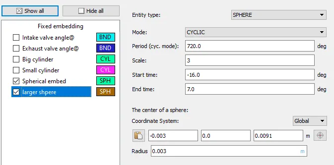
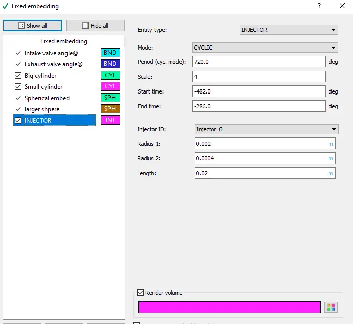
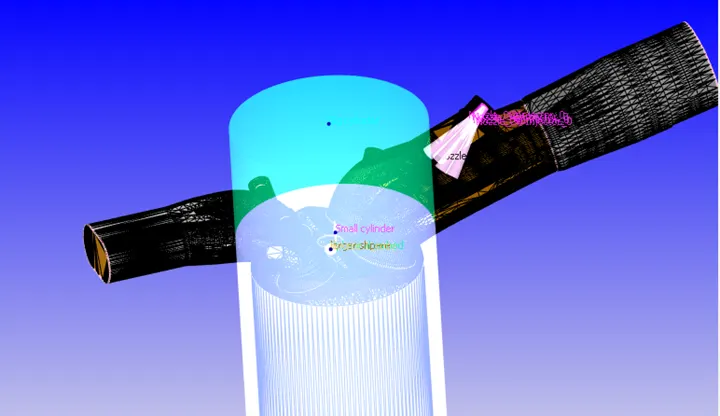
IN ADDITION TO NO HYDRO SIMULATION THE FOLLOWING FIXED EMBEDDING NEEDS TO BE ADDED

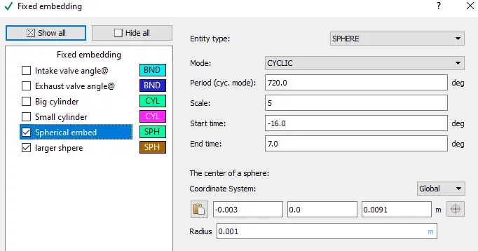
ADAPTIVE MESH REFINEMENT

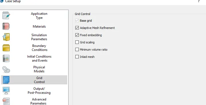
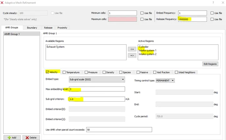
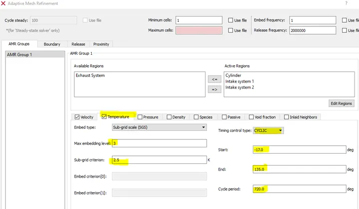
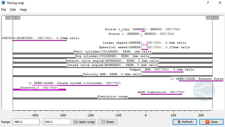
TIMING MAP – RIGHT CLICK ADAPTIVE MESH REFINEMENT

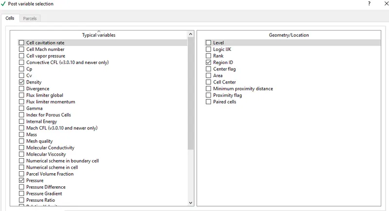
9. Post-Processing:

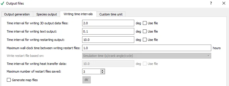
10. Output Files:

3. RESULTS AND DISCUSSION:

PLOTS:

1.Pressure plot

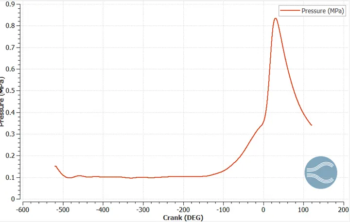
Inference: It is depicted fromt the plot that compression pressure increases & high at start of combustion

2. Mean Temperature Plot

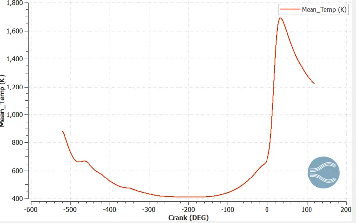
Inference: Mean Temperature is high at the start of combustion process and reaches a maximum value of 1700K

3. Heat Release Rate

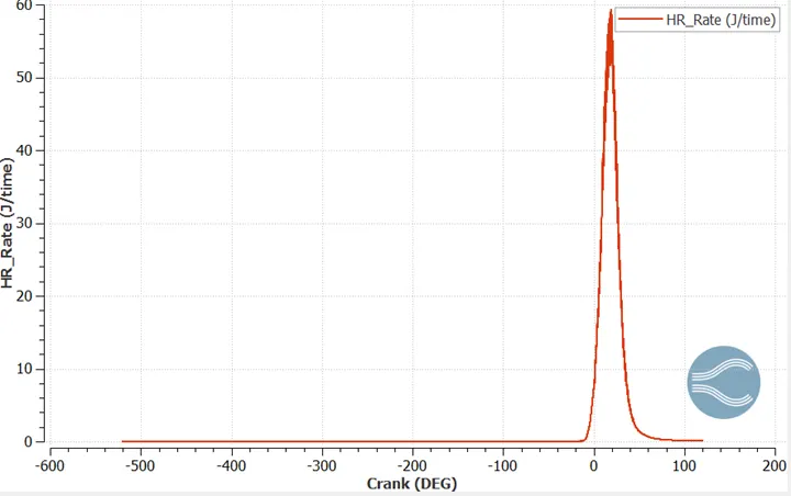
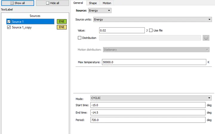
Inference: It is envisaged from the graph that Heat release rate increases on the start of combustion process and decreases at the end of cycle. Since we have specified heat source for the model at that point heat release is maximum.

4. Emission

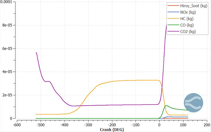
Inference: It is envisaged from the graph that CO pollutant is comparatively higher to other pollutants. CO can be reduced by installing Aftertreatment devices to meet the emission standards.

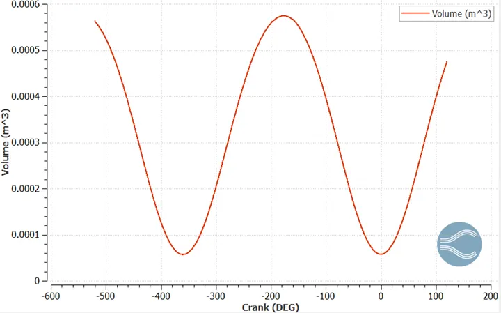
Inference:

PARAMETERS	VALUE	UNIT
Max Volume	0.000574	m^3
Min Volume	0.0000575	m^3

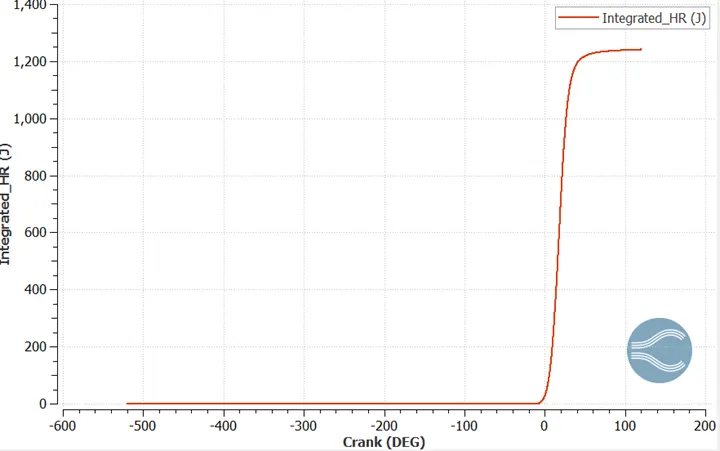
Inference:

Total Heat released by combustion

1241.04

Joules

From Graph

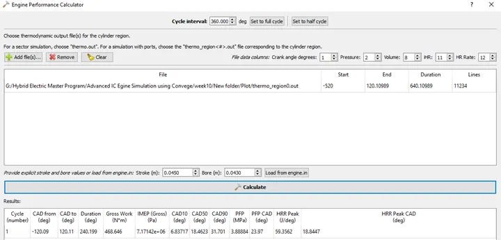
Work done	468.646	Joules	From engine performance Calculator
Duration	240.199		From engine performance calculator

The following queries are answered with detailed formulae in table below:

1. What is the compression ratio of this engine?

2. Calculate the combustion efficiency of this engine

3. use the engine performance calculator, to determine the power and torque for this engine.

Compression Ratio	PARAMETERS	VALUE	UNIT	FORMULA
	Max Volume	0.000574	m^3
	Min Volume	0.0000575	m^3
	Compression ratio	9.982608696		= Max Volume/Min Volume
		=10:1
Fuel Calculations
	RPM	3000	RPM
	RPS	50	RPS	=RPM/60
	DPS	18000	degrees/sec
	Time Per Degree	5.55556E-05	sec/degree	=1/DPS
	Time Per 720 degrees	0.04	sec/cycle	=Time per degree*720
	Fuel flow rate	7.50E-04	kg/sec	Given
	Fuel Mass per cycle	3.00E-05	kg/cycle	=fuel flow rate *timeper 720 degrees
Combustion Efficencey
	Calorific Value of Fuel	44000000	J/Kg
	Amount of Fuel	0.00003	kg/cycle	=Fuel mass per cycle
	Total Heat content of fuel	1320	J/kg	=Amount of fuel*Calorific Value
	Total Heat released by combustion	1241.04	Joules	From Graph
	Combustion Efficiency	94%		=Total heat released by combustion / Total heat content of fuel
Engine Power & Torque
	Work done	468.646	Joules	From engine performance Calculator
	Duration	240.199		From engine performance calculator
	Time per 240.199 degree	0.013344389		=Duration*Time per 720 degree/720
	Power	35119.33022	J/Sec or watts	=workdone/Time
	Pi	3.14
	Torque	111.85	Nm	=Power*60/(2*Pi*N)

4. Why do we need a wall heat transfer model? Why can't we predict the wall Temperature from the CFD simulation?

Performance and emission of an engine is affected by heat transfer. Near Wall measurement is generally used under CFD simulation but there will be some heat loss due to temperature gradient across wall. For accurate prediction of engine heat transfer, wall temperature models are useful for accomplishing heat transfer from the hot gases to all the engine parts, also to the coolant and lubrication oil. It is clear that in PFI engine simulation computational time is large due to complex geometry and solving of both Navier’s stokes and heat transfer equation when we consider the heat transfer effect between fluid and solid surface. Thus, Wall transfer models give more preference to heat transfer and less preference to fluid motion and reactions.

5. What is the significance of ca10, ca50 and ca90?

ca10	10% of the combustion take place & represents the start of ignition
ca50	50% of the combustion take place & represents the end of air-fuel mixture combustion
ca90	90% of the combustion take place & represents the end of combustion.

Animation:

Youtube Link

https://youtu.be/GlNplb_FDb0

https://youtu.be/FuRofKzmlAM

4. CONCLUSION:

The problem Full- hydro simulation by surface preparation and boundary flaggig using Converge CFD and post process the results using Paraview was simulated and below learnings were made successfully.

• Surface preparation or Geometry clean up involving eliminating errors like intersection, open edges, normal orientation and non manifold edges were studied
• Boundary Flagging and valve & piston motion simulation
• Combustion efficiency of engine was calculated.
• Compression ratio and wall heat transfer model were studied
• Power and torque was calculated using engine performance calculator.
• Importance of ca10, ca50 and ca90 were studied