PFI Engine - Full Hydro Simulation
PART 1 - PFI Engine - surface Preparation, Boundary Flagging & No-Hydro Case Setup
Introduction:
After post-processing, the No-Hydro setup, and verifying the case parameters run as specified, part 2 of this project involves full hydrodynamic simulation including the combustion and spray modeling. This study is done to evaluate the emissions such as NOx & soot produced during the combustion and understand the performance parameters of the engine such as power, efficiency, maximum temperature attained in the combustion chamber. The project begins with spray modeling, combustion modeling & details of SAGE in Converge Software.
Objectives:
- Setting up the Spray model (Injectors & Nozzles)
- Combustion Modelling
- Adaptive Mesh Refinement
- Evaluation of emission characteristics and Engine Performance parameters.
Physical Setup:
- At first, liquid parcels of IC8H18 are added into the domain from the Parcel Simulation tab (Pre-defined Liquid), where the properties of liquid fuel are available and the same is added in the Species list for Parcel.
- The setup in this project is different from the Part-1. Here, full hydrodynamic simulation is performed.
- For the Physical setup, the following models are selected. (Spray, Combustion, Turbulence, Source models)
- Finally, AMR and embedding are incorporated in the Grid control section.
- Then, the model will be ready for running the simulation.
CASE SETUP:
Surface preparation and Boundary flagging including the creation of events and regions can be referred from PART 1. Here, Spray modeling, Combustion modeling, and Source modeling are explained.
Spray Modeling:
Converge uses state of art models for spray processes involving liquid atomization, drop breakup, collision & coalescence, turbulent dispersion & drop evaporation in terms of liquid sprays. Converge uses a Lagrangian solver to model discrete particles and Eulerian solver to model the continuous fluid domain. Lagrangian specification of the flow field is a way of looking at fluid motion where the observer follows an individual fluid parcel as it moves through space and time. Plotting the position of an individual parcel through time gives the pathline of the parcel. The Eulerian specification of the flow field is a way of looking at the fluid motion that focusses on specific locations in the space through which the fluid flows as time passes. The eulerian cell center is fixed while the lagrangian parcels move. Heat, momentum & mass transfer occur between the discrete and continuous phases via source terms in transport equations.
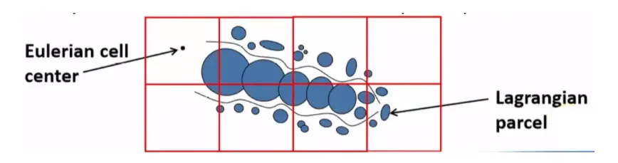
Parcels are introduced into the domain at the injector, which presents a group of identical drops with the same radius, velocity, and temperature. The parcel is the basic unit converge solves instead of drop. Parcel undergoes several physical processes like a primary breakup, secondary breakup, drop, drag, collision & coalescence, and evaporation.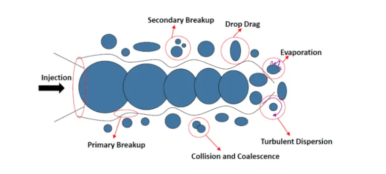
Evaporation Model:
The spray evaporation that takes place needs to be considered and for that converge uses certain standard pre-created models such as Frossling, Chiang, or with boiling. In this project, the Frossling model is used and it does not need to provide the particular equations as Converge takes care of it. Converge asks for evaporation source to simulate multi-component vaporization. The source used in this project is "Source all base parcel species" which denotes multi-component liquid species evaporate into the base species.
As the evaporation source is specified, the maximum radius of ODE droplet heating needs to be specified as well, its basically a temperature discretization parameter which will control if drop temperature is uniform or radially varying. If the drop radius exceeds maximum value the converge assumes a radially varying temperature or else uniform temperature distribution is assumed.
Spray Penetration and Distribution:
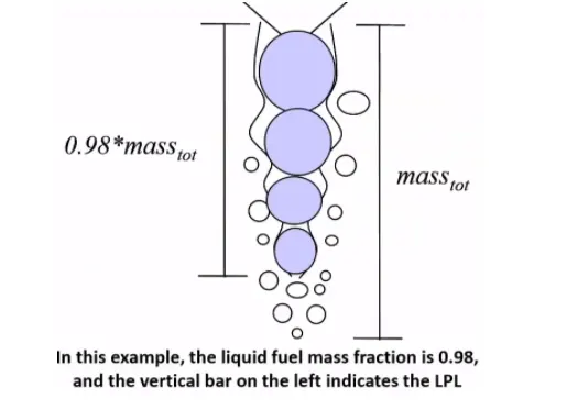
Converge writes the liquid and vapor penetration lengths at each output interval, it calculates vapor penetration length for each nozzle. For each cell that meets the criteria that fuel vapor mass fraction exceeds the user-specified value or cell size does not exceed user-specified bin size, converge calculates the center of the nozzle to the center of the cell.
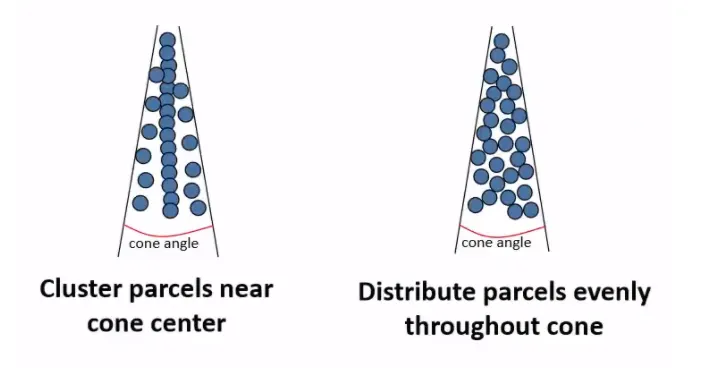
The parcel distribution is done in two ways where the parcels are either distributed evenly throughout the cone or clustered near the center of the cone. Depending upon the requirement either distribution can be selected, for this project, even distribution is selected.
Collision/Coalescence & Drop Drag:
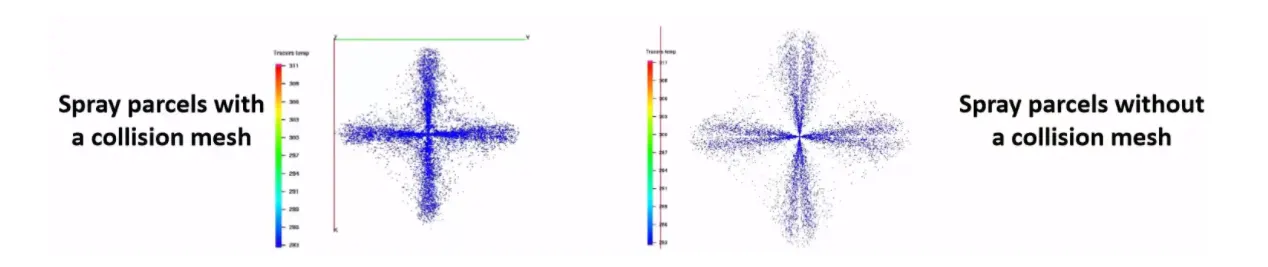
If in a spray simulation parcels collide with parcels only in the same cell, it can lead to grid sensitivity, which is why converge has an adaptive collision mesh to reduce the grid sensitivity, Once collision mesh is checked, the parcels can collide across grid cells, requiring no additional mesh or any other setup. In this project, it is done using a standard NTC collision model & dynamic drop drag calculates the drag coefficient to account for variation in drop shape as shown in spray breakup. In the figure shown below, it is observed that parcels with collision mesh look more reasonable & natural, Othe drop options are spherical drop drag & No drop drag.
Injector & Nozzle
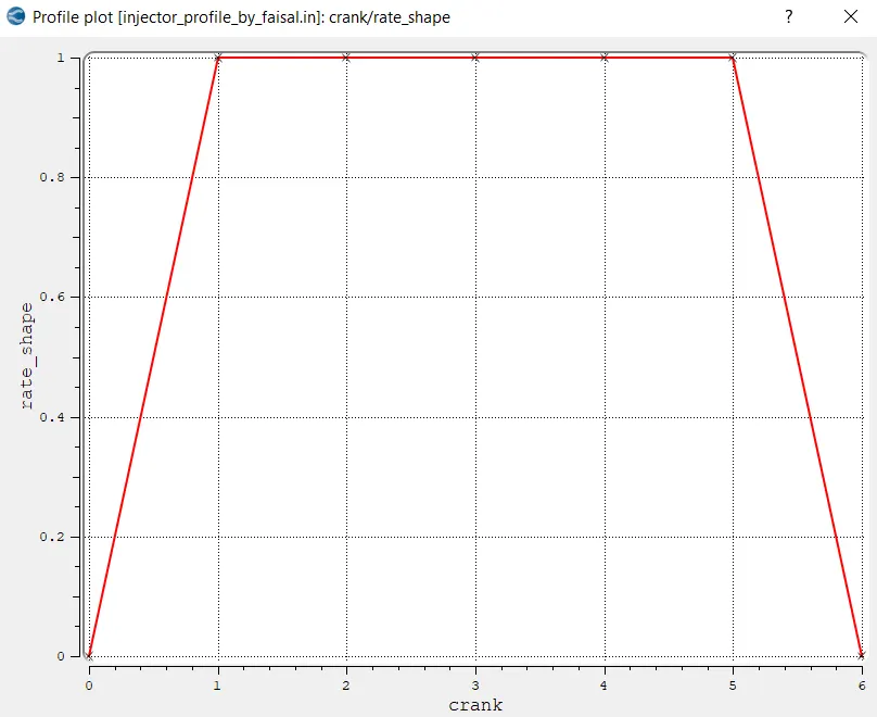
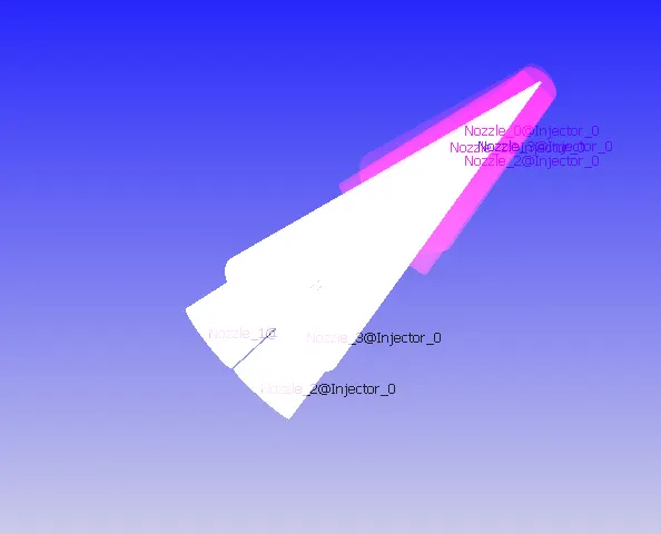
Once the spray breakup & parcel modeling is done, injectors and nozzles need to be specified in their locations, models, radius, etc, In this project, there are 4 nozzles in one injector. This is done as per the engine manufacturer's requirement based on the amount of fuel and speed at which the fuel has to be sprayed inside the chamber. The injector has a rate profile where its rate vs crank is determined (normalized for injection duration) is as shown below.
The fuel is specified for this injector as IC8H18 with mass fraction 1 as fuel is sprayed through the injector. Kelvin-Helmholtz & rayleigh Taylor models are used. The discharge coefficient recommendation for gasoline PFI - correlation for Cv - 0.8 is set.
Nozzles are added at the injector where nozzle parameters are mentioned such as diameter, injection mass & duration, radius, and spray cone angle as well as co-ordinates of the nozzle.

| Parameters | Input | ||||||||||||||
| General | |||||||||||||||
| Parcel Distribution | Distribute Parcels evenly throughout the cone | ||||||||||||||
| Turbulent Dispersion | O'Rourke model | ||||||||||||||
| Drop Evaporation | Use evaporation model | ||||||||||||||
| Frossling Model | 2-source all base parcel species | ||||||||||||||
| Collision/Breakup/Drag | |||||||||||||||
| Model |
|
||||||||||||||
| Injectors | |||||||||||||||
| Nozzles |
|
Nozzle Location:
| Center | Align Vector | |
| Nozzle 0 | 0.0823357 0.00100001 0.07019 | -0.732501 0.210489 -0.647408 |
| Nozzle 1 | 0.0823357 -0.00099999 0.07019 | -0.732501 -0.210489 -0.647408 |
| Nozzle 2 | 0.0823357 -0.0004 0.07019 | -0.5 -0.2 -0.647408 |
| Nozzle 3 | 0.0823357 0.0003 0.07019 | -0.5 0.2 -0.647408 |
The above nozzles are of diameter 0.00025 m and 0.000125m circular cone radius.
Combustion Modelling:
Combustion facilitates the energy transfer in the engine. Converge contains detailed chemistry solver and simplified combustion models. In the present project, we will be using SAGE detailed chemical kinetics solver.
SAGE:
The SAGE detailed chemistry solver is a general combustion model used to solve the detailed chemical kinetics in the combustion process. It can accurately model ignition and laminar flame propagation. It uses local conditions to calculate reaction rates based on the principles of chemical kinetics. Also, determines kinetically limited phenomenon of engine knock and emissions. It requires a CHEMKIN-formatted input fils to solve the reaction rate ODEs. The ODE solver used is called as CVODE solver. SAGE couples with transport solver via source terms in the species transport equations.
A chemical reaction mechanism is a set of elementary reactions that describe an overall chemical reaction. The combustion of different fuels can be modeled. SAGE calculates the reaction rates for each elementary reaction while the CFD solver solves the transport equations. Given an accurate mechanism, SAGE (in addition to AMR) can be used for modeling many combustion regimes (ignitions, premixed, mixing-controlled). You can use SAGE to model either constant volume or constant pressure combustion.
In each time step, the chemistry solver calculates the new species mass fractions immediately prior to solving transport equations. The change in species mass fractions is treated as a source.
`(∂barrhotildeY_m)/(∂t)+(∂barrhotildeu_jtildeY_m)/(∂x_j)=∂/(∂x_j)(barrhoD_t(∂tildeY_m)/(∂x_j))+ color(red)(tildedotω_m)`
The red color term is the source term. Detailed mathematical modeling can be found in Converge 3.0 manual.
As this is the most detailed solver, solving it in every cell can be expensive, time-consuming. Converge has accelerating options that require increasing minimum cell temperature and min HC species mole fraction to reduce the number of cells in which combustion calculations are performed. Using start time and end time to limit SAGE to a specific time interval and can limit SAGE operation to a specific region. Other options include setting resolve only if temperature changes by a specified value. Using analytical jacobian to pass an analytically calculated jacobian to the solver. SAGE also reduces time by using multizone modeling where it groups cells into bins for which options are provided in Converge.
| Parameter | Input | ||||||||||||
| Model | SAGE detailed Chemistry Solver | ||||||||||||
| General | IC8H18 fuel | ||||||||||||
| Activation Timing |
|
||||||||||||
| SAGE Parameters |
|
||||||||||||
| Adaptive Zoning |
|
Source Modeling:
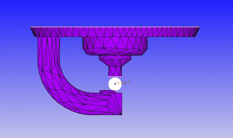
Two sources are created at the same location at different times and with different intensities to obtain realistic ignition in the combustion chamber.
| Parameters | Source1 | Source2 |
| Source | Energy | Energy |
| Source Units | Energy | Energy |
| Value (J) | 0.02 | 0.02 |
| Mode | Cyclic | Cyclic |
| Start Time [deg] | -15.0 | -15.0 |
| End Time [deg] | -14.5 | -5 |
| Period [deg] | 720 | 720 |
| Shape | Sphere | Sphere |
| Center & Radius | (-0.003,0,0.0091) & 0.0005 | (-0.003,0,0.0091) & 0.0005 |
From the above table, it is clear that two sources are superimposed between -15 to -14.5 [deg] i.e., during this duration 0.04J of energy is released due to spark ignition and for the rest of the duration i.e., -14.5 to -5 [deg] 0.02J of energy is released due to the aftereffect of spark.
Fuel Mass Calculation:
We need to input the total mass of fuel injected per cycle in Kg, which is calculated as shown below.
Given that the mass flow rate of fuel is 7.5e-4 kg/s and RPM of 3000, it is possible to calculate mass flowing per cycle for a period of 720 [deg].
RPM is converted to RPS (rotations per second) which is further converted to DPS (degrees per second). From DPS we can determine the time taken for 720 [deg] and the mass flow in Kg can be obtained.
3000 RPM = 3000/60 RPS = 50 RPS
50 RPS = 50*360 DPS = 18000 DPS
Time taken for rotation by one degree is 1/18000.
Time per degree = 1/18000 DPS = 5.55e-5 s.
Time for 720 degrees = 5.55e-5 * 720 = 0.04s
So, the total mass of fuel injected per cycle is 7.5e-4 [kg/s] * 0.04 [s] = 3e-5 kg
Grid control:
Apart from the fixed embedding used in Part-1 further refinements are added to the Grid control.
Adaptive Mesh Refinement:
Adaptive mesh refinement is a method of adapting and enhancing the grid dynamically depending upon the variation in the second-order variation of parameters.
Velocity SGS
It is permanent with an embedding level of 3 for SGS of 1 m/s.
Temperature SGS
It is cyclic with an embedding level of 3 for SGS of 2.5K after the fuel is injected into the cylinder.
The formula used is as below:
`"Grid Size" = "Base Grid" / 2^("embedding layers")`
Fixed Embedding:
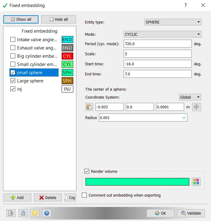
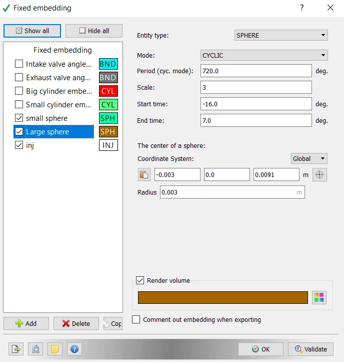
Apart from the fixed embedding used in Part 1 further embedding is added near the spark plug and injectors.
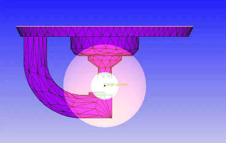
Fixed embedding small sphere
Fixed embedding large sphere
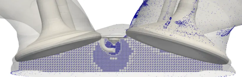
The effect of embedding near the Spark plug is as shown below.
Fixed embedding for injectors
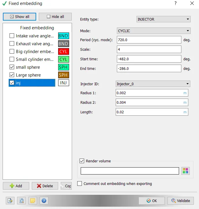
The embedding zones for the injector are as shown below.
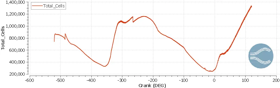
Total Cells:
It shows how the cells are adapted according to the combustion activities and effectiveness of AMR and fixed embedding.
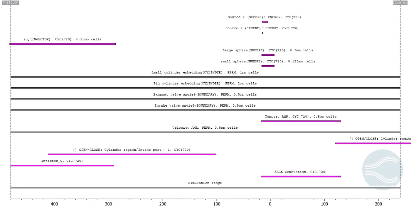
Timing Map:
The timing map is like a pathway that lays out all simulation timing details into something like process charts which displays which process is activated at a particular time. It is a handy tool to verify the activities in one place.
Results & Discussion:
After completing the modeling of the case, the simulation was run using the CYGWIN command line terminal on a 16 core machine and it took 1 week to finish the entire simulation. Once it is simulated the data is post-processed using ParaView. On the cluster, the simulation was run between -520 to 120 [deg].
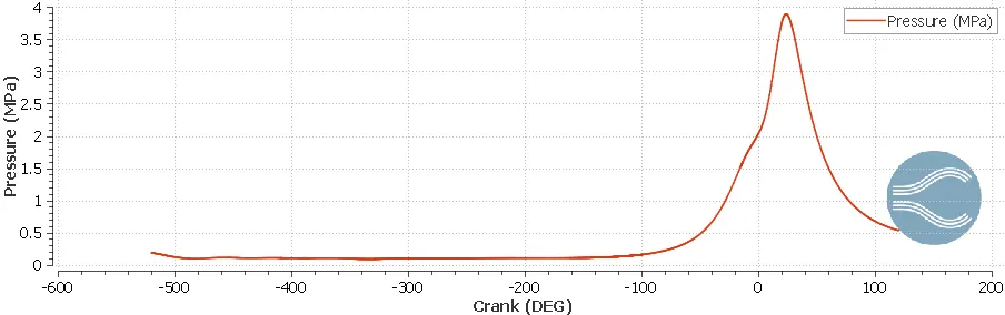
In-Cylinder Pressure:
The cylinder pressure contains different values at different strokes of the cylinder, the highest of which is observed in the combustion/Expansion stroke. This stroke is where the spark plug ignites the air-fuel mixture, creating very high pressure. This is where the engine power is generated. The peak pressure is 3.884 MPa.
Volume & Compression Ratio:
The volume vs crank angle graph plotted in the cylinder region is as shown below.
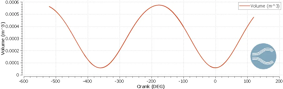
The maximum volume obtained is 0.0005742195 (m^3) and the minimum volume is 0.000057029438(m^3).
Hence the compression ratio is as defined below.
`"Compression Ratio" = "Maximum Volume"/"Minimum Volume" = 0.0005742195/0.000057029438 =10.06875`
PV Plot:
The SI engine follows a typical otto cycle as can be observed from the PV plot. The work done can be calculated by determining the area under the curve.
`W= intP.dV`
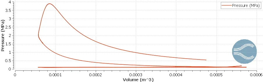
Converge provides an inbuilt engine performance calculator in which all the performance terms can be calculated.
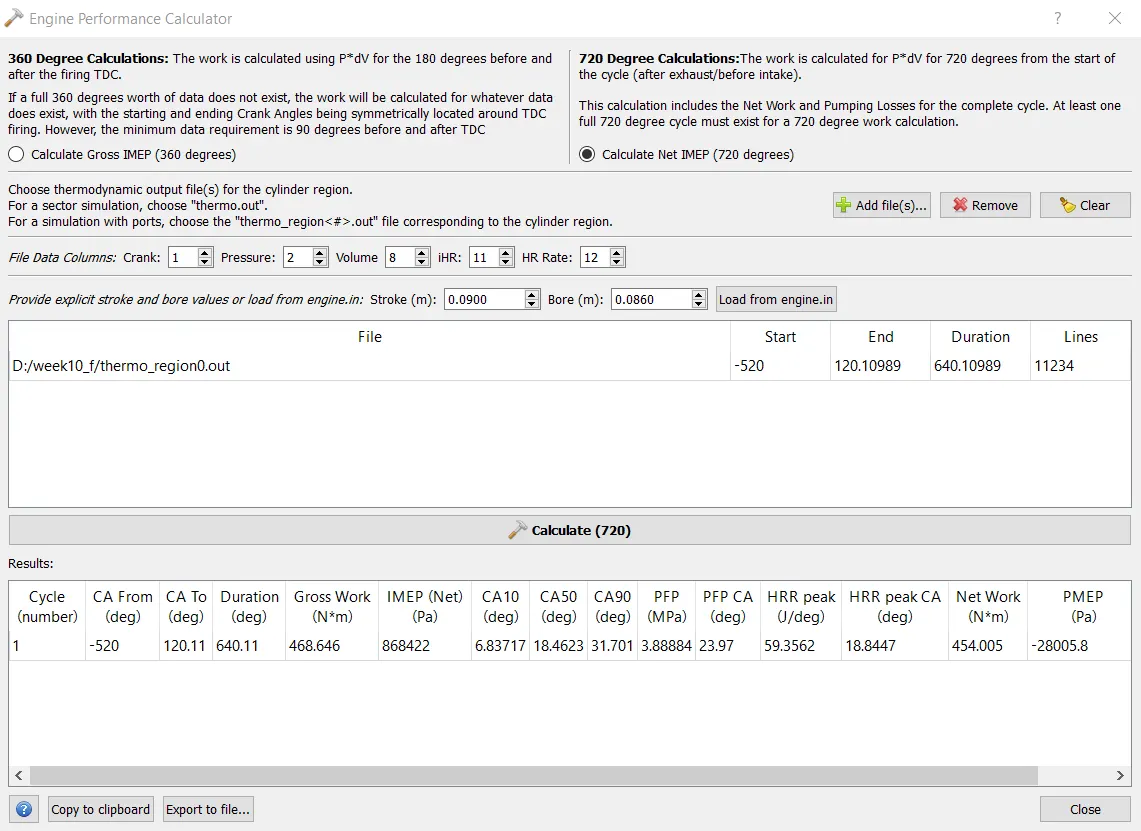
The total gross work obtained is 468.646 Nm.
The duration of the cycle is 640.11 [deg]. From the above, we got that the duration for each degree is 5.55e-5 s.
For 640.11 [deg] we get, 0.035526s
The net power generated (work/time) during the cycle can be calculated as 468.646/0.035526 i.e., 13191.63 W.
Torque can be obtained from the formula below:
`P = (2 pi N tau )/60`
`tau = (P * 60) /(2*pi*N)`
`tau = (13191.63 *60)/(2*pi*3000) = 41.99 Nm`
Heat release rate & combustion efficiency:
Heat release & Integrated heat release is plotted as shown below. It gives the amount of heat i.e., total amount of heat released from combustion process. From the total heat release in the combustion chamber, the combustion efficiency of the engine can be determined.
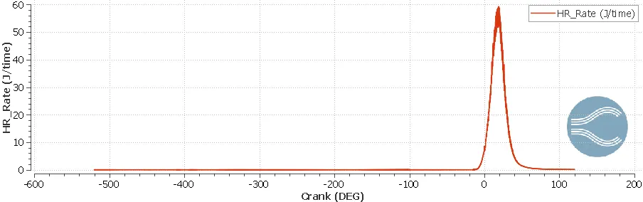
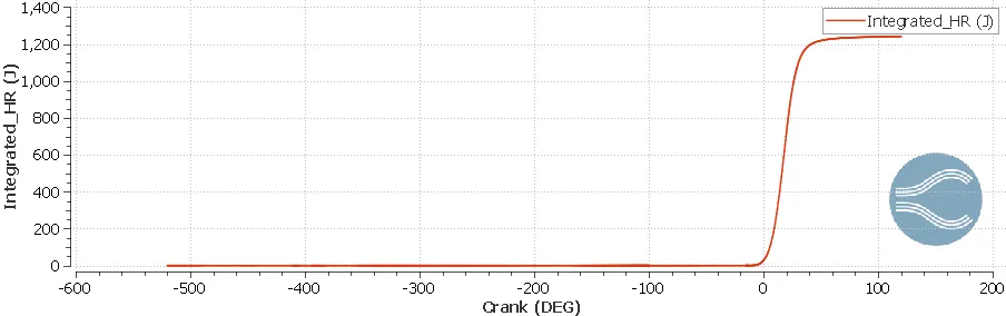
Combustion efficiency is defined as the ratio of total heat energy released by the burning of fuel to the total energy content of fuel mass in a cycle.
Mass of fuel injected = 3e-5 kg
Calorific value of fuel = 44e6 J/kg
Integrated heat released = 1250 J
`eta = "Heat Released"/(m.LHV) = 1241/(3e-5*44e6)=0.94015`
Hence, combustion efficiency is 94.015%
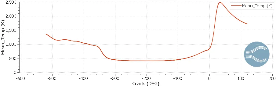
Mean Temperature:
The mean temperature data is used for the design of the liner and thermal analysis of the engine.
The animation below shows how the energy from the spark is propagated in the combustion chamber.
The animation below shows how the temperature of parcels is varied and vaporized as well as the temperature along the cut plane.
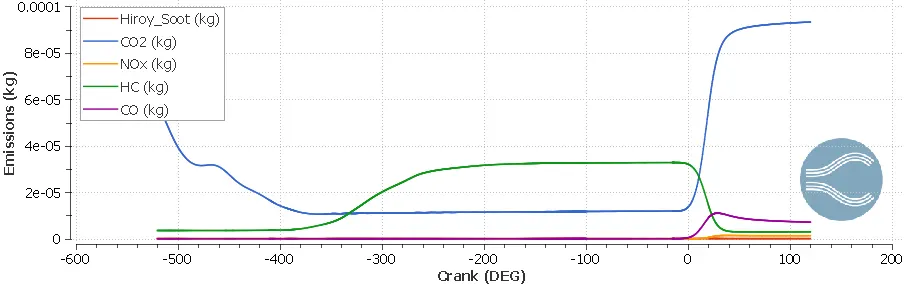
Emissions:
The major cause of emissions is due to rich/lean mixtures or unburnt hydrocarbons. The emissions of concern are unburnt hydrocarbons (HC), oxides of carbon, nitrogen & sulfur and soot particles. The emissions are produced in the combustion region which is then released from the exhaust port.
Spray Parcels:
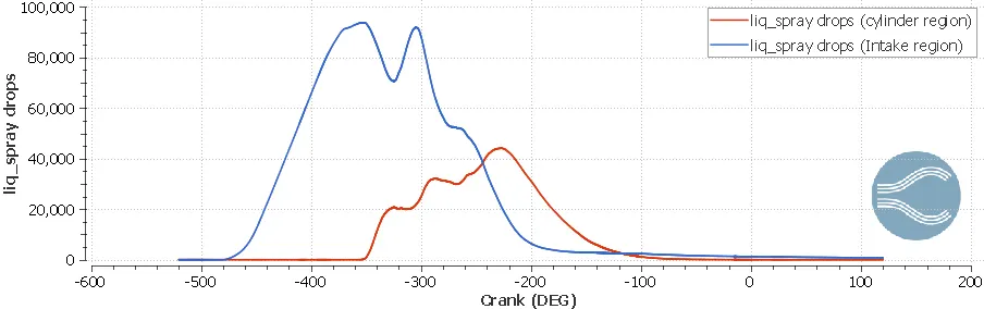
Spray parcels are injected from nozzle to intake port and then to the cylinder region with the aid of the intake valve. When the spray parcels are reached into the cylinder region half of the parcels are atomized as can be seen from the figures below. Few of the parcels get trapped in the intake port before all the parcels reach the cylinder region and it was taken care by giving the appropriate initial conditions in that region.
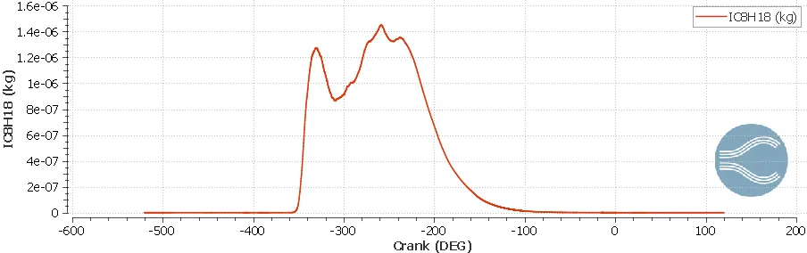
Spray Parcels Velocity Animation:
The inlet parcels in the velocity animation can be seen as they inject with high velocity there velocity reduces when it strikes the inlet valve and then is released into the cylinder region and few of the parcels are trapped in the intake port. These parcels upon reaching the cylinder region get vaporized and combusted in the later stages.
Neccessity of wall heat transfer models:
Accuracy is important to predict engine performance. Modeling of heat transfer and wall temperature is a critical task of any engine thermodynamic model. In addition to the fluid domain, engine design needs to consider the materials of the engine. In addition to this simulation, we need to perform the CHT or thermal analysis of the engine model wherein the temperatures of the solid domains need to be predicted accurately. In order to predict the wall temperatures, we need to use well-defined wall heat transfer models to obtain accurate results.
Significance of CA10, CA50 & CA90:
CA refers to the crank angle and the number suffixed to it represents the percentage of fuel burnt. For Eg. CA50 means crank angle at which 50% of combustion (fuel burnt) takes place. In general, CA10 represents the onset of combustion, CA50 represents combustion phasing and CA10-90 represents burn duration. At these corresponding crank angles, combustion data and performance parameters are recorded and are used for validation with experimental results.