Hyperelastic Material Modelling and validating simulation with Experimental data using LS-Dyna

AIM: To calculate the Mooney Rivlin and Ogden material constant then compare and validate the Hyperelastic material with the help of experimental data.

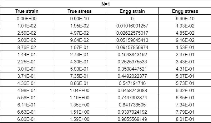
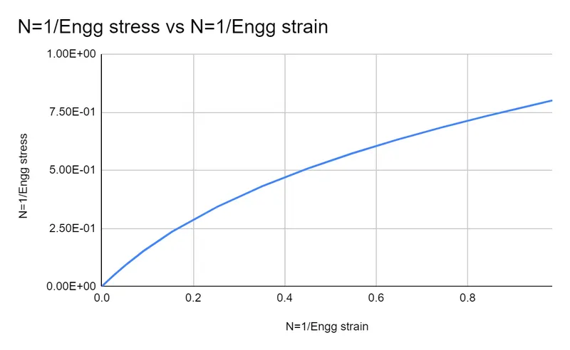
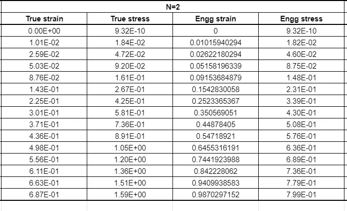
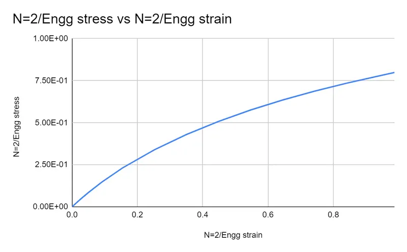
ABSTRACT: In this challenge, we are going to model the hyperelastic material by calculating the Mooney and Rivlin constant and comparing the simulation result with the experimental data(Engg. strain-stress) are given (shown below).

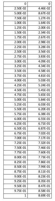
OBJECTIVE: The workflow is as following:

• Define the curve data(engineering stress-strain) from the experiment to the model file.
• Extract the Mooney Rivlin and Ogden material constant.
• Set the deck Boundary condition for the tensile test for the hyperelastic material.
• Compare the D3HSP data with the experimental data to get the best fit order curve constant
• Define the constant for different N(order) values to get the simulation results for the true strain and stress values.
• Compare the simulation data with experimental data.

THEORY:

A general material is elastic up to 0.2 to .002% of the strain it starts behaving plastically or nonelastic right after that.

Hyperelastic Material:

1. It is a highly elastic material in the sense that all deformation can be recovered.
2. Ideal elastic material (no permanent deformation).
3. undergoes large deformations.
4. The stress-strain relationship is derived from strain energy density function.
5. A non-linear relation between stress-strain

there are many material models available for hyperelastic material which are defined by the N state of constant.

• N=0 for defining curve constant without actual defining the curve (C10,C01,C11,C20,C02... etc)
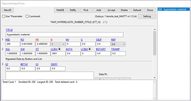
• N=1 for defining curve with Mooney-Revlin constant.
• N=2 and n=3 for Ogden constant.

As the material has to account for both nonlinear and large deformation therefore it is not described as a stress-strain curve rather described in the terms of strain energy per unit volume as a function of stretch.

eg. Rubber, foam and, adhesives

METHODOLOGY:

1. Get the Stress-strain curve from material testing: [kind of data extracted, what is the best data available, the behaviour of the complex material]
2. Check the fitness of the curve to the maximum correlation :[ compare fit from different option]
3. Finalization parameters& determine format:[ simulation should be validated with the test data]

PROCEDURE:

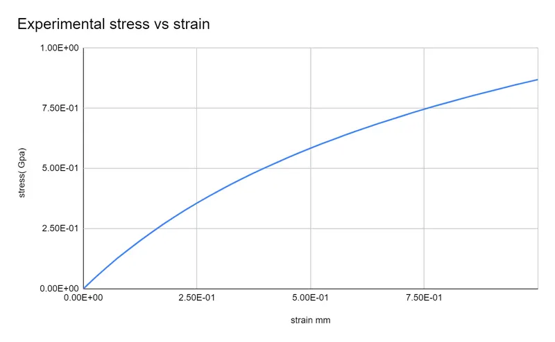
1) Plot the data(Stress-strain) check the material behaviour and type.

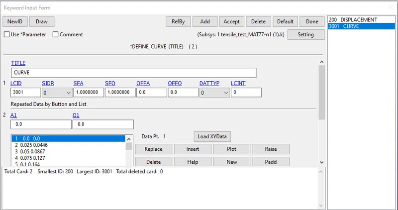
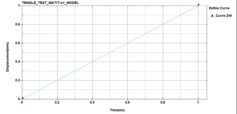
2) Define the curve data in LS-post inside the *DEFINE_CURVE as shown below

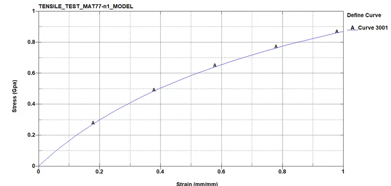
3) Boundary conditions

a) Prescribed Motion Set

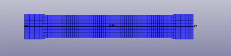
AS we have a 100 % strain i.e dl = l i.e 145 mm therefore we need to give a displacement of 145 mm to attain a displacement of strain value 1

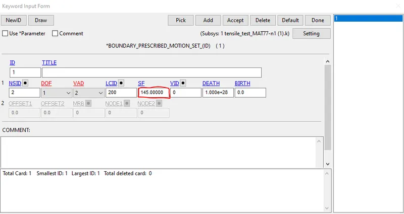
Make the node-set for the extreme left edge nodes to assign them the Prescribed Motion (displacement)

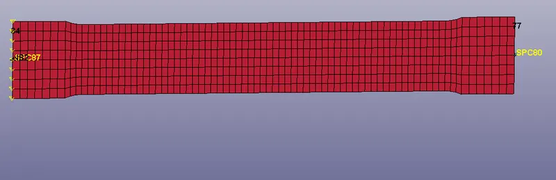
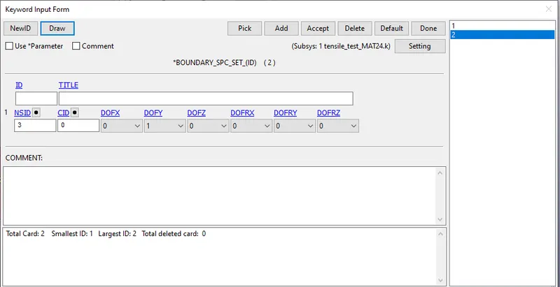
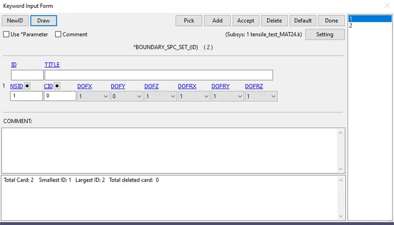
b) SPC (Arrest the DOF for the part to give the real tensile test situation)

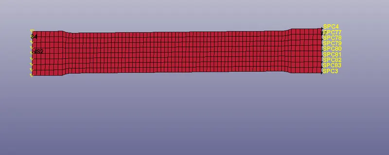
Define the SPC for the mid nodes on each side (left & right) to arrest the DOF in the Y direction (shown below)

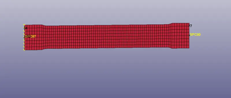
Define the SPC for the right extreme nodes on the right side to arrest the DOF in all the direction except in the Y direction (shown below)

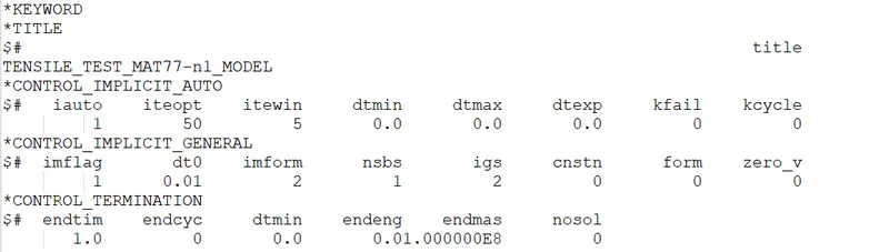
4) Control and Database card setup

Control card

Database Card

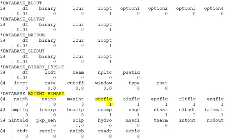
NOTE: Define the DATABASE_EXTENT_BINARY CARD wit the strflg value =1 to get he strain values at the output for the element.

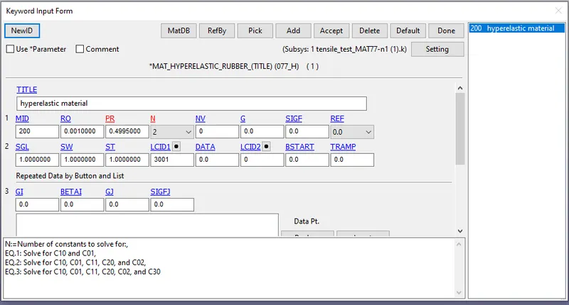
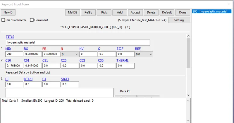
5)Define Material card : MAT 077Hyperelatic material card setup and calculation

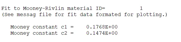
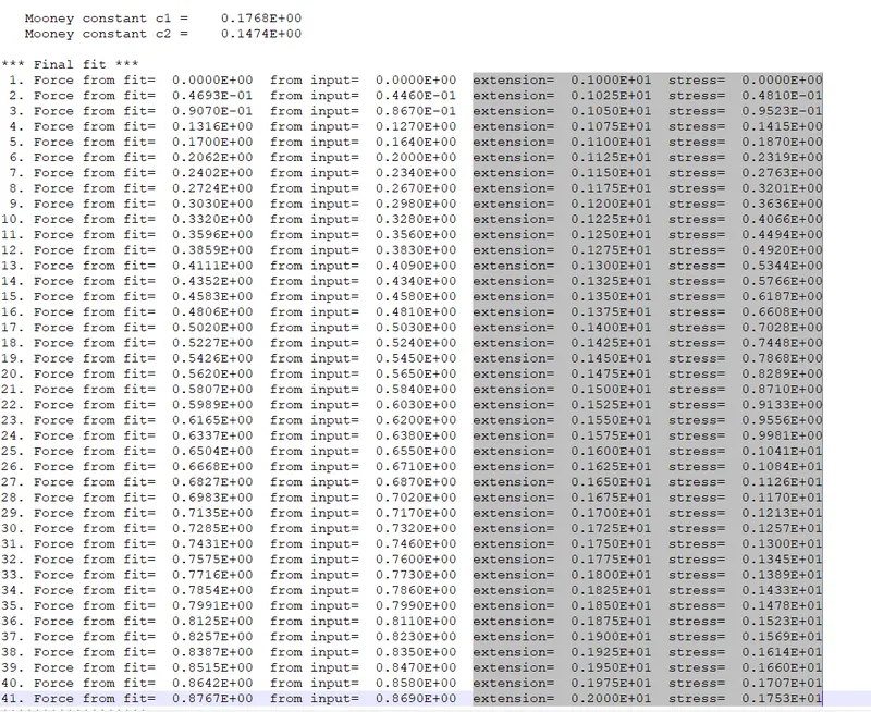
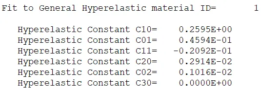
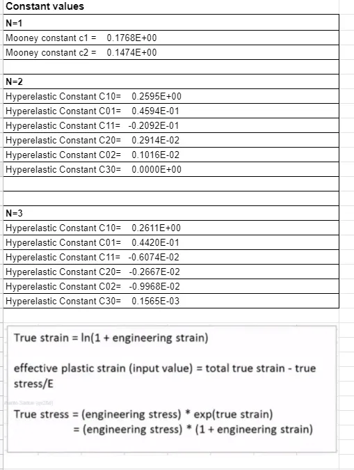
Calculated constant from D2HSP file.

1) For N=1

2)For N=2

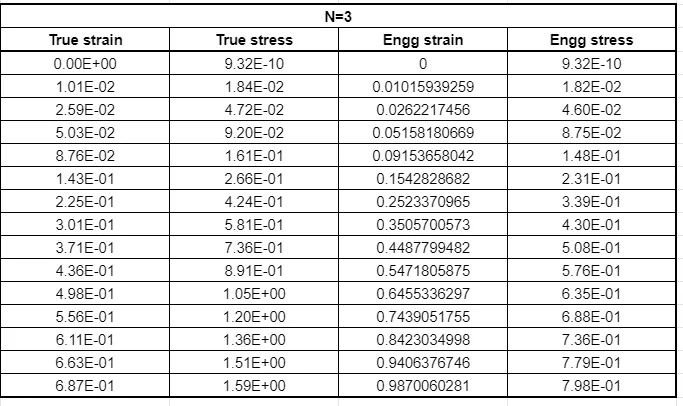
3) For N=3

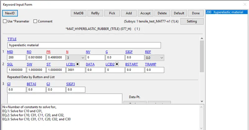
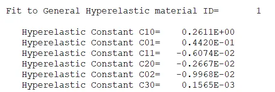
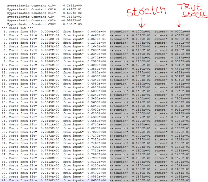
once you input the material parameters with different N=1,2,3 then you will get different constant values that have to save to avoid calculation every time run the file from the defined curve.

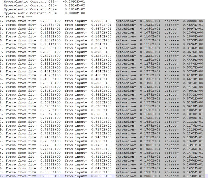
just below the **Final fit** the last two column tells about the stretch and true stress which need to be modified using the equation

1. `lamda= 1+epsi_(engg)` where `lamda`is stretch
2. `sigma_(true)=sigma_(engg)(1+epsi_(engg))`

NOTE: you need to look at the D3HSP file to get the constant values and Final fit data for stretch and true stress values.

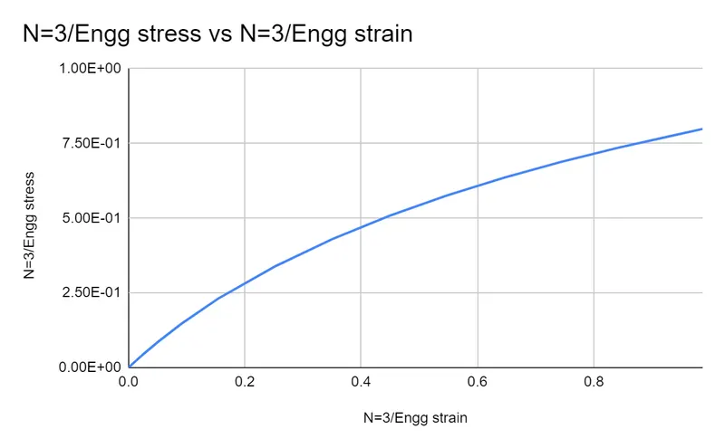
Engineering stress and strain computation and comparison from D3HSP file

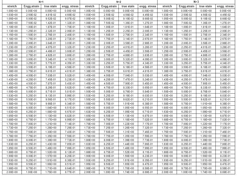
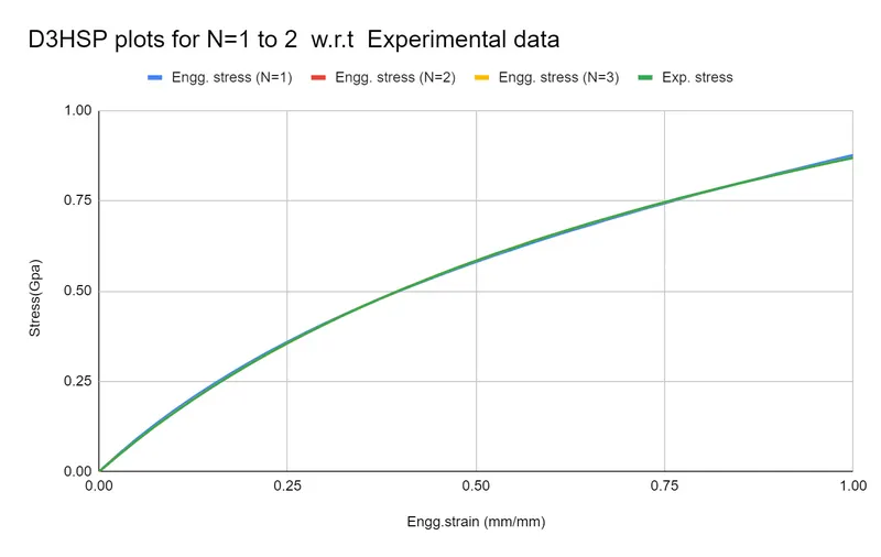
The above plot shows that very closed correlation of the experimental data with the computed polynomial curve for N= 1,2 and, 3

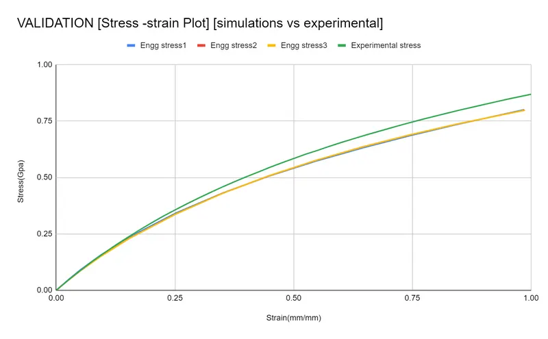
VALIDATION of the computed data with experimental data

Now we will take the N=0 and feed the constant value obtained from different N values to the Material card parameter.

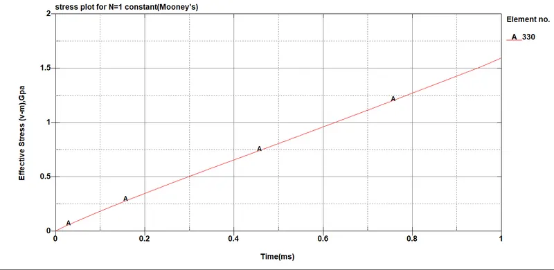
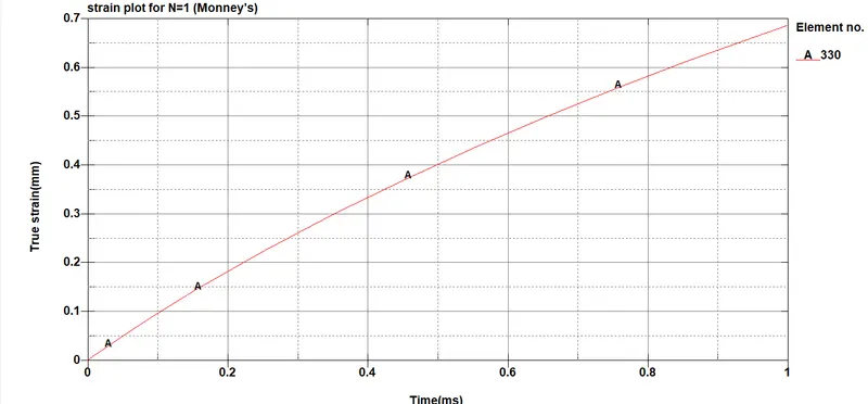
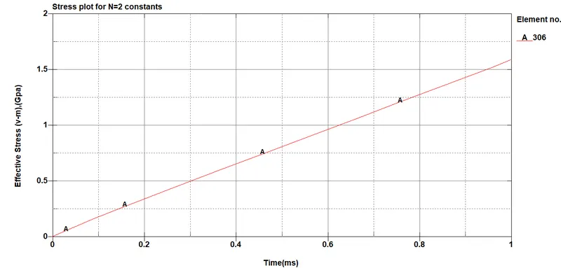
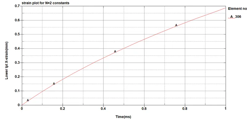
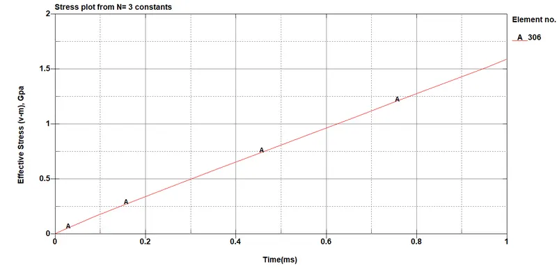
After running the solver we will open the binary file and check for the stress wrt time (V-M stress ) and strain wrt time(lower strain values in x) values and save them and then cross plot them as stress-strain plots for each case of n value constant.

from N= 1 constant

From N= 2 constant

From N=3 constants

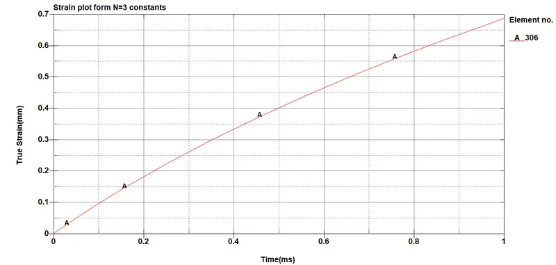
RESULTS:

Validation Results:

As we can see from the comparison the resulting curve we got from the simulation with different polynomial constant shows a slight variation with the experimental data which is within the acceptable zone as this is for a very small strain problem for a hyperelastic material. We are accounting this problem and stress-strain plot for a very early stage of the strain which has very non-linear behaviour, therefore, we are able to see a very smooth simple curve. The actual experimental stress developed are a bit more than simulation results for the same strain levels. it could have shown much deviation for the different degree of the polynomial for large strain problems.

ANIMATION

Effective stress(true stress)

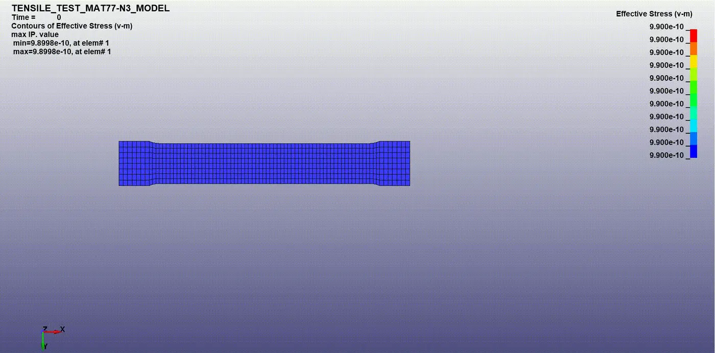
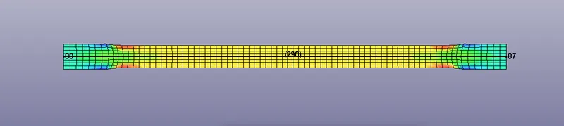
Elongation of Dogbone during the simulation

1)Start of simulation ->At T=0, length = 145mm

2)End of simulation-> At T= 1 ms, length= 290 mm

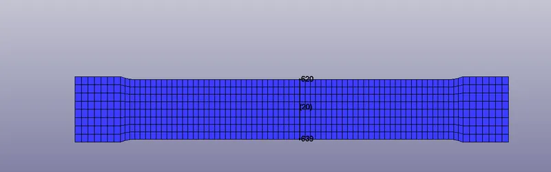
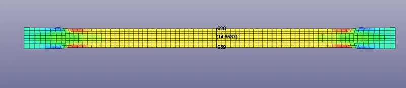
Reduction in Area

1) At the start of the simulation(width= 20mm)

2) At the end of the simulation(width=14.63mm)

CONCLUSION:

1. The strain produced is as per the given data i.e. 1 as the final length of the dogbone is twice the original length.
2. The reduction in area is 5.37 mm^2 at the end of the simulation.
3. As this is a small strain problem for a hyperelastic material therefore we get almost very similar fit with all the degree of polynomial"(N=1,2,3).
4. There is slight variation in the simulation curve and the experimental curve but within the acceptable limits. but this may be significant if the strains are very large.
5. The stress and strain obtained from the Ls-post simulation are True stress and strain values they must be carefully modified and covered into equivalent comparable forms.
6. we get the material curve constant values inside the D3HSP file and below the **final fit** last two-column for stretch and true stress data.