Week - 10 Hyperelastic Material Models
Assignment 10
1. Introduction
In this assignment, a discussion will be made about two different formulations for modelling rubber: Mooney-Rivlin and Odgen. Based on provided experimental data obtained from a tensile test, the parameters involved in both theories were calculated and an approximated model for each theory was created. Then, these approximated models will be implemented in LS-Dyna and the results from the experimental data, model data and simulation data will take place.
2. Experimental Data
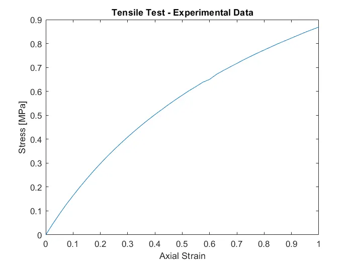
An image containing the data obtained from a tensil test was provided. The following figure shows a graph of that data.
3. Mooney-Rivlin
In the Mooney-Rivlin formulation, the Strain Energy Density function is given by:
`W = \frac{U}{V} = \sum_{i,j = 0}^{n} C_{ij}(I_1-3)^i(I_2-3)^j \ \ \ \ \ \ \ \ \ \ \ \ (1)`
Where U is the Energy Density function. For the simple example of a specimen subjected to an axial load P, as shown in the following figure, the U function is given by: `U = \int_0^x P dx \ \ \ \ \ \ \ \ \ \ \ \ (2)`

Developing the previous expression, and knowing that the tip displacement (x) is given by `x = \varepsilon L`(L being the length of the specimen and `\varepsilon` the axial strain), we obtain:
`W = \frac{U}{V} = \frac{1}{V}\int_0^xPdx = \frac{1}{V}\int_0^\varepsilonPLd\varepsilon = \frac{L}{V}\int_0^\varepsilonPd\varepsilon = \frac{1}{A}\int_0^\varepsilonPd\varepsilon = \int_0^\varepsilon \frac{P}{A}d\varepsilon = \int_0^\varepsilon \sigma d\varepsilon \ \ \ \ \ \ \ \ \ \ \ \ (3)`
Where `\sigma` is the normal stress at the thinnest cross-section of the specimen.
This means that, if it is possible to obtain an expression of W that depends only on `\varepsilon`, we can differentiate it to obtain an analytical expression for `\sigma` depending on `\varepsilon`.
It will be assumed that the maximum possible values for i and j are 1, therefore:
`W = \frac{U}{V} = \sum_{i,j = 0}^{n} C_{ij}(I_1-3)^i(I_2-3)^j = C_{00} + C_{10}(I_1-3) + C_{01}(I_2-3)+C_{11}(I_1-3)(I_2-3) \ \ \ \ \ \ \ \ \ \ \ \ (4)`
Where:
`I_1 = \lambda_1+\lambda_2+\lambda_3\ \ \ \ \ \ \ \ \ \ \ \ (5)`
`I_2 =\lambda_1\lambda_2+\lambda_1\lambda_3+\lambda_2\lambda_3\ \ \ \ \ \ \ \ \ \ \ \ (6)`
`\lambda_1 = \varepsilon + 1= \varepsilon_1 + 1\ \ \ \ \ \ \ \ \ \ \ \ (7)` Stretch ratio in the axial direction (direction 1)
`\lambda_2 = \varepsilon_2 + 1\ \ \ \ \ \ \ \ \ \ \ \ (8)` Stretch ratio in direction 2
`\lambda_3 = \varepsilon_3 + 1\ \ \ \ \ \ \ \ \ \ \ \ (9)`Stretch ratio in direction 3
The strains in the directions that are orthogonal to the axial direction are related to `\varepsilon_1` by the Poisson coefficient `\nu`(For rubber materials, this coefficient is approximately 0.5):
`\varepsilon_2 = \varepsilon_3 = -\nu\varepsilon_1\ \ \ \ \ \ \ \ \ \ \ \ (10)`
`ith the previous expressions, it is possible to confirm that W can be written as a function of `\varepsilon_1`
This material represents a singular case in which the value of `I_1` is constant and independent from `\varepslion_1`, due to the fact that `\varepsilon = 0.5`
`I_1 = \lambda_1 + \lambda_2 + \lambda_3 = \varepsilon_1 + 1 + \varepsilon_2 + \varepsilon_3 + 1 = \varepsilon_1 - \nu(\varpesilon_1\times2)+3 = 3`
This means that the second and fourth term of the right-hand-side of equation 4 will always be null.
The calculation of the `C_{ij}` parameters was based in the experimental data. To calculate them, two points were considered:
3.1. `\varepsilon = 0; \sigma = 0 MPa`
For this point, the following values for the stretch ratios are obtained:
`\lambda_1 = \lambda_2 = \lambda_3 = 1` (Since there is no deformation)
`I_1 = 3`
`I_2 = 3`
Now, replacing these values in equation 4:
`\int_0^\varepsilon\sigma d\varepsilon = C_{00} \Leftrightarrow C_{00} = 0`
3.2. `\varepsilon = 1; \sigma = 0.869 MPa`
In this point, the values for the strains in directions 1, 2 and 3 are the following:
`\varepsilon_1 = 1 `
`\varepsilon_2 =varepsilon_3 = -\nu\times\varepsilon_1 = -0.5`
for the stretch ratios are the following:
`\lambda_1 = 2`
`\lambda_2 = 0.5`
`\lambda_3 = 0.5`
The values for the `I` parameters are:
`I_1 = 3` and `I_2 = 2.25`
Replacing in equation 4:
`W = C_{01}(I_2-3) = -0.75C_{01}`
3.3. Stress-strain curve determination
Alternatively, W is also equivalent to:
`W = \int_0^{1}\sigmad\varepsilon = 0.5371 {MJ}/{m^3}` (Integral solved using the experimental data and MatLab)
By combining the two expressions above, it is possible to calculate `C_{01}`:
`W = -0.75C_{01} = 0.5371 \Leftrightarrow C_{01} = -0.7161`
We can now obtain the analitical expression for `\sigma`:
`W = -0.7161(I_2-3)=\int_0^\varepsilon\sigmad\varepsilon \Leftrightarrow -0.7161(\lambda_1\lambda_2+\lambda_1\lambda_3+\lambda_2\lambda_3-3) = \int_0^\varepsilon\sigmad\varepsilon \Leftrightarrow`
`\Leftrightarrow-0.7161((\varepsilon_1 + 1)(\varepsilon_12 + 1)+(\varepsilon_1 + 1)(\varepsilon_3 + 1)+(\varepsilon_2 + 1)(\varepsilon_3 + 1)-3) = \int_0^\varepsilon \sigma d\varepsilon \Leftrightarrow`
`\Leftrightarrow -0.7161[(\varepsilon_1+1)(-0.5\varepsilon_1+1)+(\varepsilon_1+1)(-0.5\varepsilon_1+1)+(-0.5\varepsilon_1+1)(-0.5\varepsilon_1+1)-3] = \int_0^\varepsilon \sigma d\varepsilon \Leftrightarrow`
`\Leftrightarrow -0.7161[2(\varepsilon_1+1)(-0,5\varepsilon_1+1)+(-0.5\varepsilon_1+1)^2-3] = \int_0^\varepsilon\sigma d\varepsilon \Leftrightarrow`
`\Leftrightarrow -0.7161[-2\varepsilon_1+0.5\varepsilon_1] = \sigma \Leftrightarrow`
`\Leftrightarrow \sigma = 1.074\varepsilon_1`
3. Odgen
The generic expression for the strain energy density function is:
`W = \sum_{p = 1}^{N} \frac{\mu_p}{\alpha_1} (\lambda_1^{\alpha_1}+\lambda_2^{\alpha_1}+\lambda_3^{\alpha_1}-3)`
In this case, only one term will be used, so W is given by:
`W = \frac{\mu_1}{\alpha_1}((1+\varepsilon_1)^{alpha_1}+(1+\varepsilon_2)^{alpha_1}+(1+\varepsilon_3)^{alpha_1}-3) = \frac{\mu_1}{\alpha_1}((1+\varepsilon_1)^{alpha_1}+(1-\nu\varepsilon_1)^{\alpha_1}+(1-\nu\varepsilon_1)^{\alpha_1}-3) = \frac{\mu_1}{\alpha_1}((1+\varepsilon_1)^{alpha_1}+2(1-\nu\varepsilon_1)^{\alpha_1}-3)`
Similarly to the previous case, a relation between `\sigma` and `\varepsilon` can be obtained:
`W = \int_0^\varepsilon \sigma d\epsilon \Leftrightarrow \frac{\mu_1}{\alpha_1}((1+\varepsilon_1)^{\alpha_1}+2(1-\nu\varepsilon_1)^{\alpha_1}-3) = \int_0^\varepsilon \sigma d\varepsilon \Leftrightarrow \frac{\mu_1}{\alpha_1}(\alpha_1(1+\varepsilon_1)^{\alpha_1 -1}-2\nu\alpha_1(1-\nu\varepsilon_1)^{\alpha_1-1}) = \sigma`
Now, we consider two points obtained from the experimental data to calculate the values of `\mu_1` and `\alpha_1`:
- Point 1 : `(\varepsilon,\sigma) = (1,0.869)`
By replacing the coordinates of this point in the expression above, the following expression was obtained:
`\mu_1 =\frac{0.869}{2^{\alpha_1-1}-0.5^{\alpha_1-1}}`
- Point 2 : `(\varepsilon,\sigma) = (0.5,0.584)`
Similary as it was done before, this expression was obtained:
`\frac{0.584}{1.5^{\alpha_1-1}-0.75^{\alpha_1-1}}`
By equaling both expressions above, the values for `\mu_1` and `\alpha_1` were determined:
`\alpha_1 = 1.96`
`\mu_1 = 0.814`
4. Simulation Setup
4.1. Mooney-Rivlin
The LS-Dyna formulation for this material is slighty different than the one that was used:
`W = A(I-3)+B(II-3)+C(III^{-2}-1)+D(III-1)^2`
Where `I_1 = I, I_2 = II, I_3 = III `
The variable calculated previously (`C_{01}`) corresponds to B and the value of C is zero. Therefore, A can be calculated as:
`A = \frac{C-B}{0.5} = 1.432`
The values of A and B are used as the input for the MAT_MOONEY-RIVLIN_RUBBER.
4.2. Ogden
The order of fit of the model was set to 1. The number of terms in the series is also 1 to match the pre-analysis approach for this material. G was set to 600 which is 250-1000 times the values of SIGF (Stress limit for frequency independent frictional damping) which was set to 2 MPa, to enable frequency independent damping troughout the whole simulation. Besides that, the dimensions of the gauge and specimen were defined.
5. Results
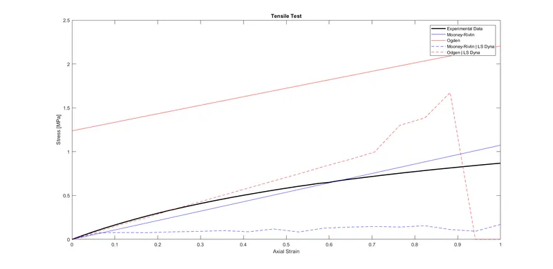
The results obtain are demonstrated and compared in the figure below. The black line corresponds to the practical data that was provided. The blue line represents the theoretical (full line) and simulation (dashed line) results obtained for the Mooney-Rivlin material. A similar representation is done in red for the Ogden material.
6. Conclusion
In general, it can be seen that there is a week correlation between the dashed and full lines in the results, this can be due to instabilities in the model, that had a more severe effect towards the end of the simulation, which is the reason why the red dashed line in the figure above had to be subjected to a correction in the last two printed time steps to avoid excessively high results to appear in the graph.
Another possible reason for the lack of correpsondence between theorectical and simulation results is the fact that the most simple formulation type was picked (the W expression had the fewest terms possible). I chose to do this to possibilitate a comparison between theorectical and simulation results. If more terms were added to the W expression, obtaining theorectical results would be more time-consuming but, on the other hand, there could be a stronger match between the simulation results and the experimental ones.