Hyperelastic Material Modelling using LS-Dyna
OBJECTIVE:
To calculate Mooney Rivlin and Ogden's material constants and compare both using stress-strain data from a Dogbone specimen tensile test with 100 percent strain.
PROCEDURE:
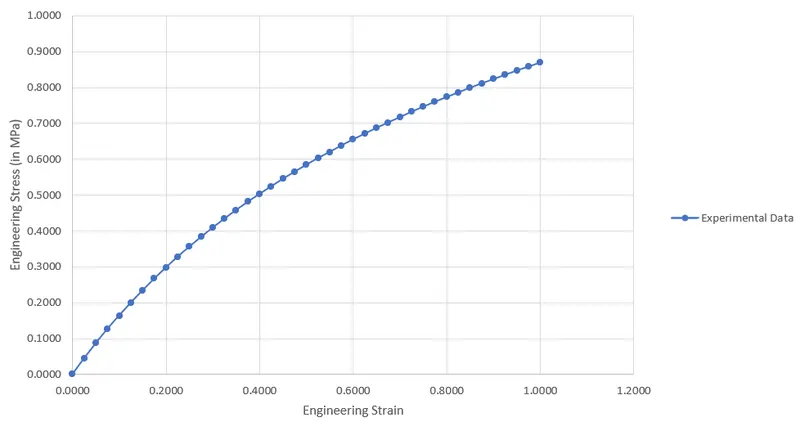
1. The given engineering stress-strain values are tabulated in excel and the values are plotted as shown in the figure below.
2. The given dogbone model is imported in the LS-Dyna PrePost
3. The boundary conditions are explained in the figures shown below.
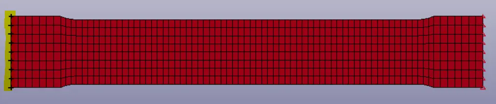
For the above-highlighted nodes, all the degrees of freedom are arrested except for translation along the y-axis.

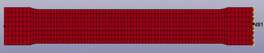
For the above-highlighted nodes, the translation along the y-axis is only arrested. This is done to achieve realistic deformation on the model.
4. For the other end of nodes, a boundary prescribed motion set is defined to apply the displacement. This is shown in the figure below.
The displacement curve ID is shown in the figure below.
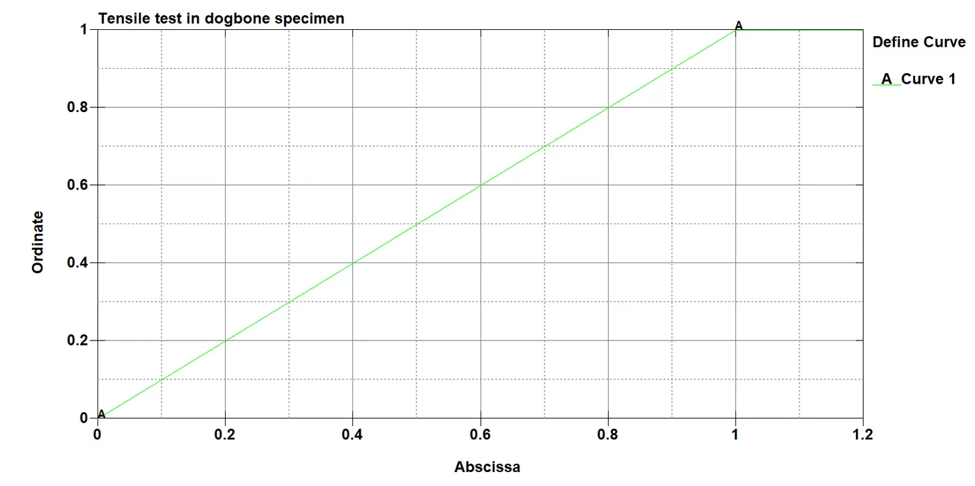
The scale factor for the displacement definition is given as 100mm.

This value is obtained from the calculation shown below. 100 percent strain equals a stretch ratio of 2.
`lambda=1+epsilon_e`
where `lambda` represents the stretch ratio
`epsilon_e` represents the engineering strain.
Therefore, 2=1+Engineering strain which implies Engineering Strain = 1
`epsilon_t = ln(1+epsilon_e)`
where `epsilon_t` represents the true strain
Therefore, true strain= ln(2) which implies
Displacement/Intitial Dimension = ln(2)
Therefore, Displacement = ln(2)*145 = 100 mm
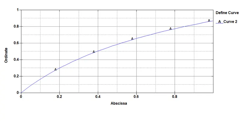
5. The material curve ID for the two materials is shown in the figure below. This is directly obtained from the tabulated excel values in step 1.
6. The material card definition for both the materials are shown in the figures below.
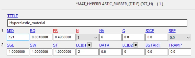
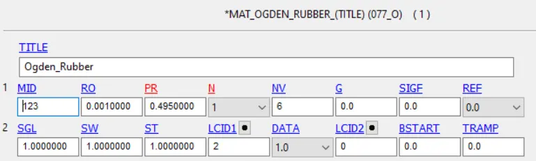
Note: The value of N is to be changed after every run (i.e., after obtaining the constants). The two material models are to be simulated separately. For validation, the value of N must be kept 0 and the obtained constants have to be plugged in to get the results.
7. The SECTION_SHELL card is defined with a thickness of 1.5 mm. The section and material cards are assigned to the part card.
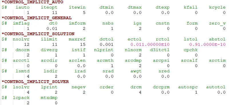
8. The *CONTROL_IMPLICIT cards are defined since this analysis can be considered as a static structural problem. The termination time is given as 1 ms. The cards are shown in the image below.
9. The necessary output requests are placed which include *DATABASE_EXTENT_BINARY and *DATABASE_ASCII and BINARY_D3PLOT.
10. The model is saved with a suitable name with a .k extension. The simulation is done using LS-Dyna Manager.
RESULTS AND DISCUSSION:
For Hyperelastic Rubber (Mooney-Rivlin constants)
1. The stress contours for different cases are shown below.
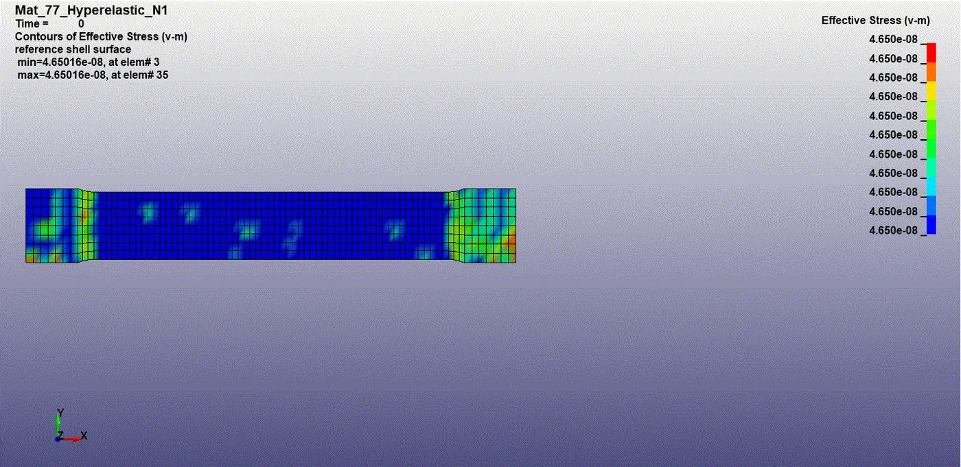
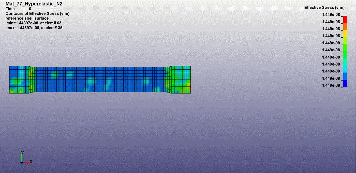
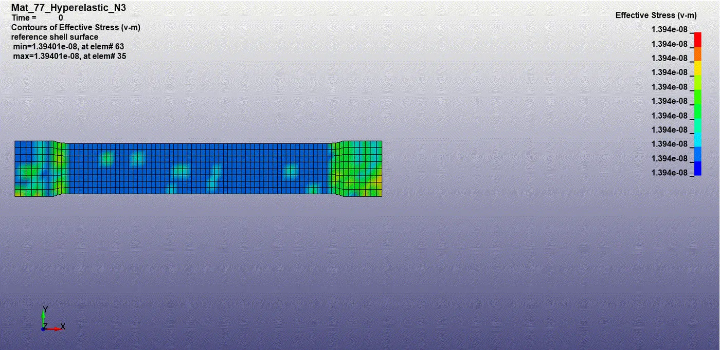
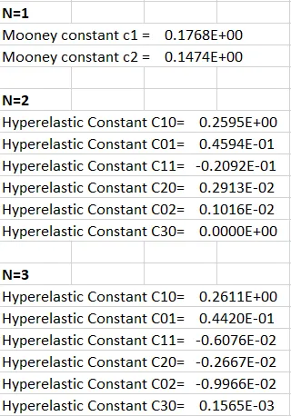
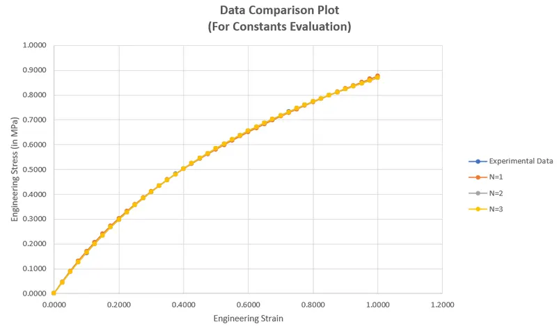
2. The following constant values are obtained for N=1,2 and 3 respectively.
3. From the d3hsp file, the values of true stress and strain are obtained and they are converted to the engineering stress and strain to compare with the experimental data. The results are shown below.
VALIDATION OF CONSTANTS OBTAINED:
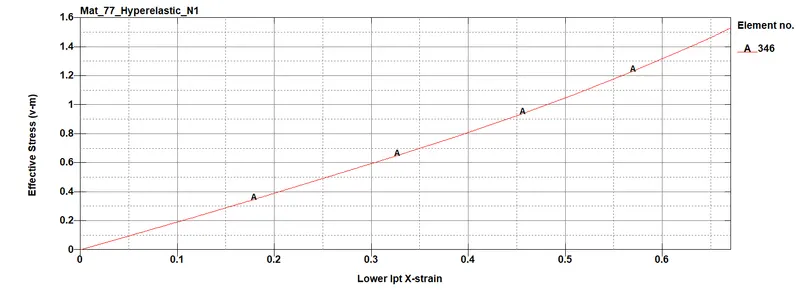
As discussed in the procedure, in the material card N is kept as 0 and the obtained constants are plugged in and the model is simulated. In this part only for N=1 constant validation procedure is explained.
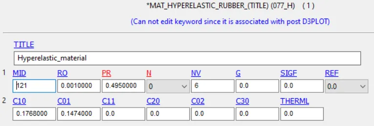
The plot obtained is shown in the figure below.
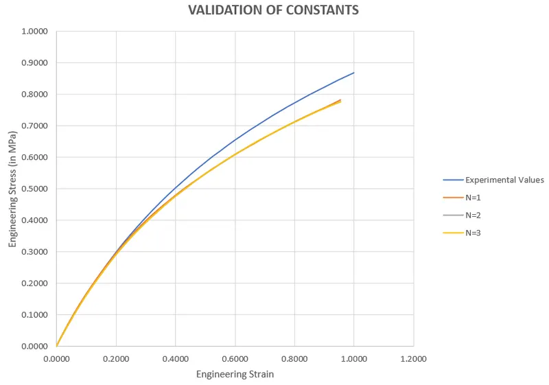
The obtained values are tabulated in excel for all three cases and results are compared with the experimental data.
For Ogden Rubber:
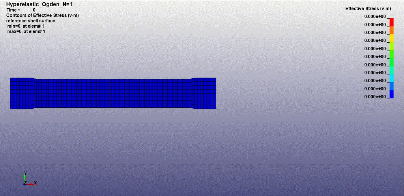
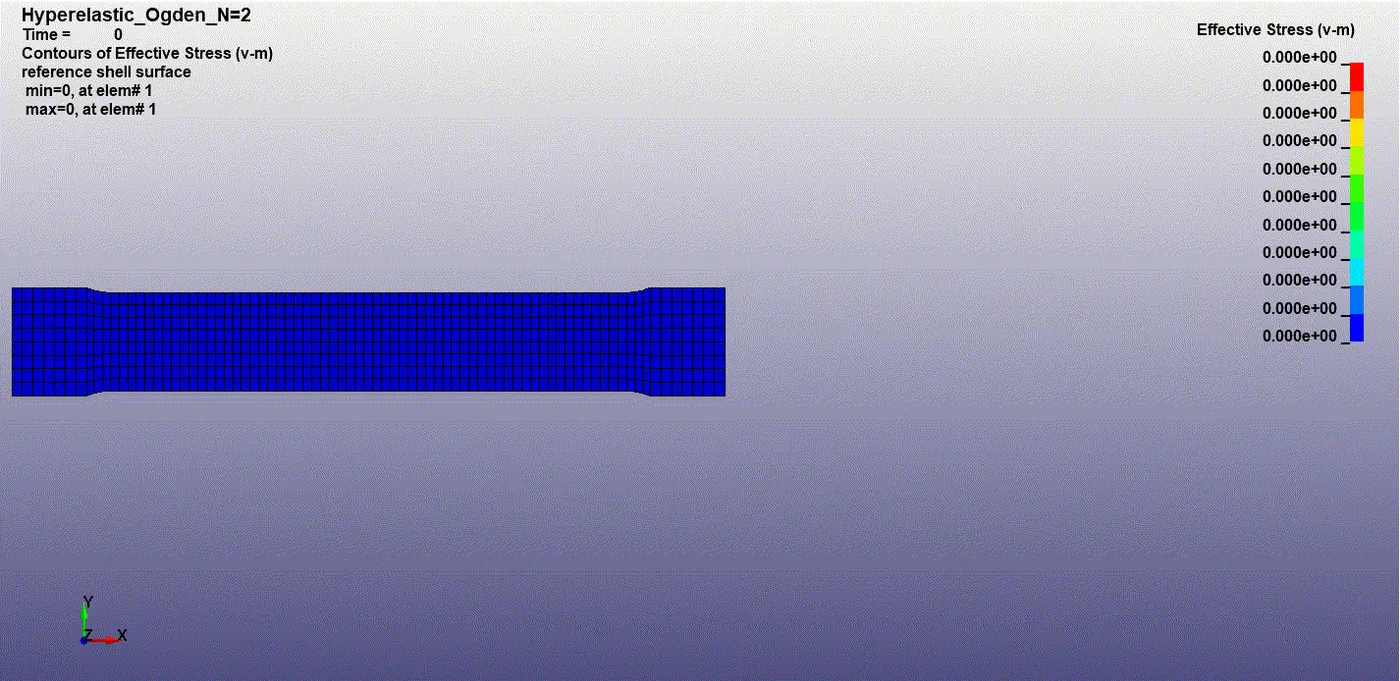
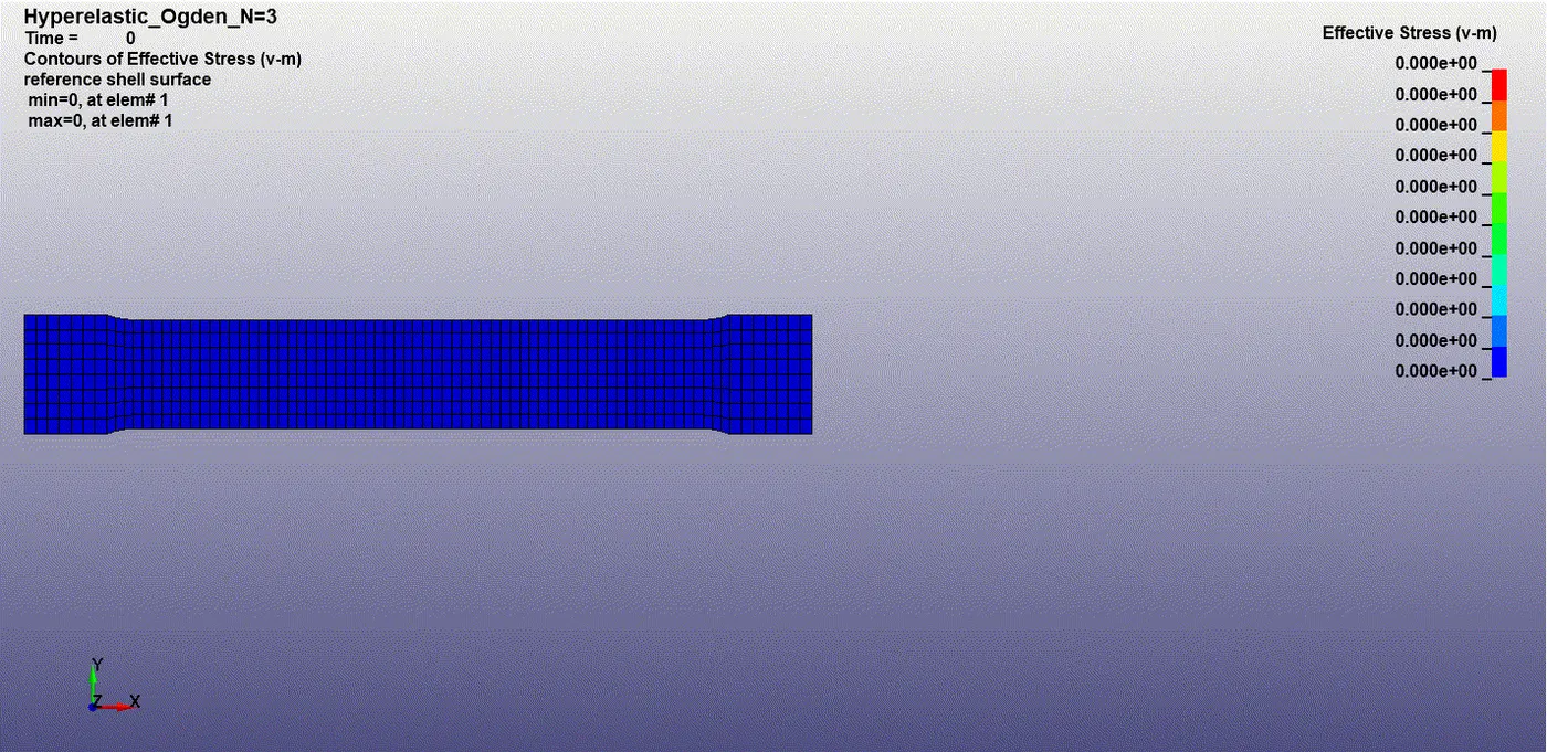
1. The stress contours for different cases are shown below.
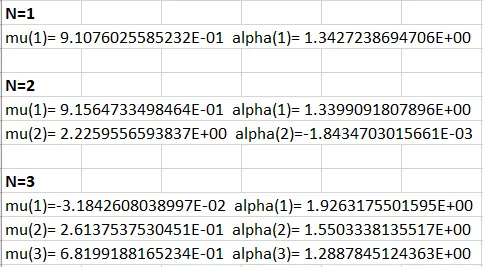
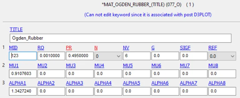
2. The following constant values are obtained for N=1,2 and 3 respectively.
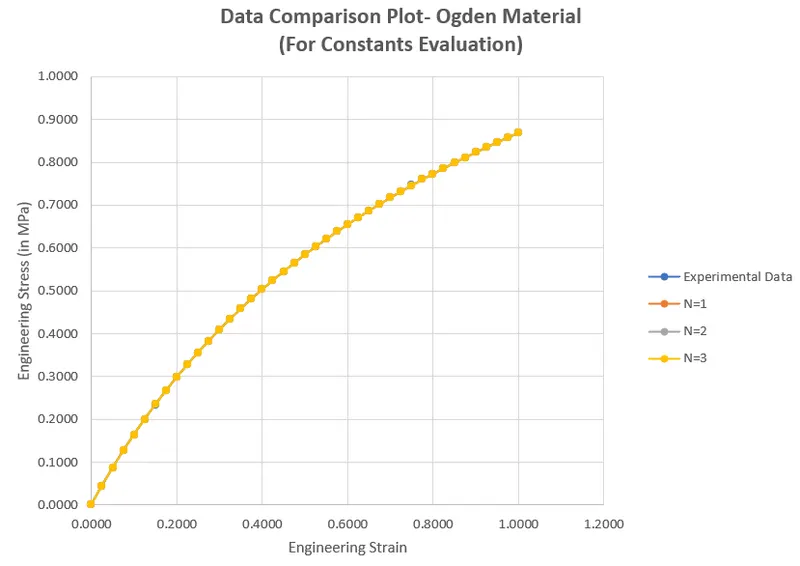
3. From the d3hsp file, the values of true stress and strain are obtained and they are converted to the engineering stress and strain to compare with the experimental data. The results are shown below.
VALIDATION OF CONSTANTS OBTAINED:
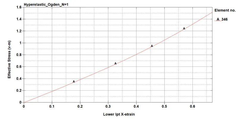
As discussed in the procedure, in the material card N is kept as 0 and the obtained constants are plugged in and the model is simulated. In this part only for N=1 constant validation procedure is explained.
The plot obtained is shown in the figure below.
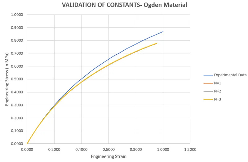
The obtained values are tabulated in excel for all three cases and results are compared with the experimental data.
Note:
1. The validation results differ from experimental data as shown in the cases above. This is because the constants are evaluated by keeping the N values as 1,2 and 3. But while validating the N value is kept as 0. This is can lead to differences in values.
2. The lower Ipt X-Strain is obtained by activating the database extent binary option. This card writes out the strain tensors.
3. In some cases, the simulation won't converge. For example, at a displacement of 145 mm, the convergence does not happen. This is because of more displacement value. By reducing the displacement suitable results can be achieved.
4. Since the loading curve is defined till a strain of 1, the true values cannot be computed to a strain of 1.
5. The element approximately at the center of the specimen must be taken for obtaining the values of stress and strain.
6. The accuracy of the material model is highly dependent on the experimental values obtained. Also, more number of simulations using various parameters has to be carried out till consistent data is obtained from the material model.
CONCLUSION:
The given experimental values are modeled using a hyperelastic material card in LS-Dyna and validated using the dogbone specimen. All the objectives in the challenge are satisfied.
Drive Link: https://drive.google.com/file/d/1lge10_8f-MQmMuFQF0og2Mi2ziK9XqeG/view?usp=sharing