Week 1- Mixing Tee

AIM

For this challenge, two versions of mixing tees are created. One longer than the other.Set up steady-state simulations to compare the mixing effectiveness when the hot inlet temperature is 36 degrees C and the cold inlet is at 19 degrees C.

Use the k epsilon and k omega SST model for the first case and based on this use a more suitable model for further cases.

• Case 1
• short mixing tee with a hot inlet velocity of 3m/s
• momentum ratio of 2,4

• Case 2
• long mixing tee with a hot inlet velocity of 3m/s
• momentum ratio of 2,4

momentum ratio = velocity at cold inlet/velocity at hot inlet

In a table compare the following values from the 2 cases

• cell count
• average outlet temperature
• number of iterations for convergence

INTRODUCTION

In industrial process engineering, mixing is a unit operation that involves the manipulation of a heterogeneous physical system with the intent to make it more homogeneous.Mixing is performed to allow heat and/or mass transfer to occur between one or more streams, components, or phrases. Modern industrial processing almost always involves some form of mixing.

A mixing tee is a type of mixing mechanism. Mixing tees utilize a specifically engineered internal geometry to efficiently mix two fluid streams into one combined stream. Mixing tees are widely used in the petrochemical, HVAC industry, etc in which two fluid streams with different physical and/or chemical properties mix together.

Hot air flowing in the main pipe is mixed with cold air flowing through a tee. The standard deviation of temperature is computed to quantity the degree of mixing. the velocity and temperature fields are also computed.The effects of the mesh size and turbulence model on results were examined.

For this, we have created two versions of the mixing tee.One of them is longer than the other. It is set up as steady-state simulations to compare the mixing effectiveness when the hot inlet temperature is 36 degrees C and the cold inlet is 19 degrees C.

SOLVING AND MODELLING APPROACH

In order to do this we need to work on the long and short tee with the following inputs:

• short mixing tee with the hot inlet velocity of 3m/s and cold inlet 6m/s
• short mixing tee with the hot inlet velocity of 3m/s and cold inlet 12m/s
• long mixing tee with a hot inlet velocity of 3m/s and a cold inlet 6m/s
• long mixing tee with the hot inlet velocity of 3m/s and cold inlet 12m/s

Hot inlet temperature 36 degrees C; Cold inlet temperature 19 degrees C

So we need to load the geometry, carry out meshing on it, provide setups, attaining solutions and the results for the mixing tee procedure.

PRE-PROCESSING AND SOLVER SETTING

In this, we are going to do the entire procedure for the mixing tee with the 2 cases individually. The procedure is as follows:

• Geometry

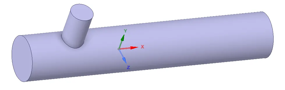
Double-click on the fluid flow(fluent) option under analysis systems. Load the CAD data for the short mixing tee by importing the CAD data option and then edit the CAD model under the space claim on the geometry. Select the edges under the volume extract tool found under the prepare window and select the edges around the circular outlet and inlets of the body. This produces the volume enclosure of the mixing tee. Hide the mixing tee and only keep the volume extract shown.

• Mesh

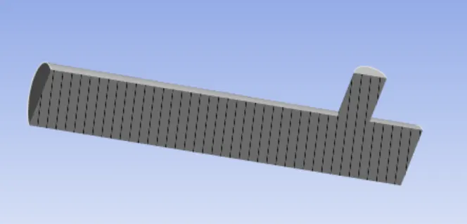
Select faces click on the face to be selected and choose the option to create a named selection and name the volumes with respective names(inlet -x, inlet - y, walls, and outlet). The element size should be 5e^-3. Use the section plane to divide the tee into equal halves.

• Setup and solution

After doing every step close those tabs and open the new tabs accordingly. In the setup window select double precision and the process should be given according to the computer system used(4).

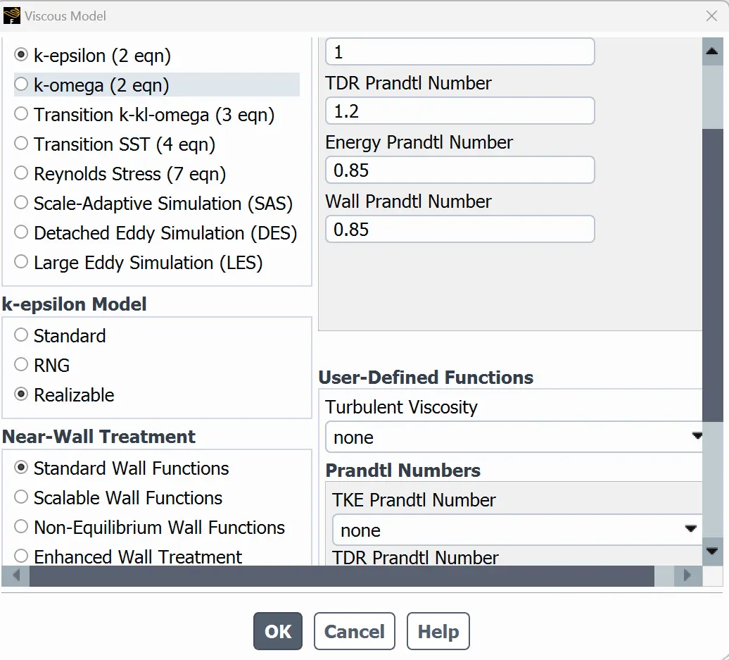
Under physics keep the following values - under time give steady, under type give pressure and under lover give absolute and give a tick to energy and under viscous model select k epsilon and k omega. Under zones select boundaries and edit for the values of velocity and temperature of the hot and cold inlets(inlet -y, inlet -x). Give the appropriate values according to the challenge requirements. Go to units under the domain window and change to temperature with C as a unit(celsius).

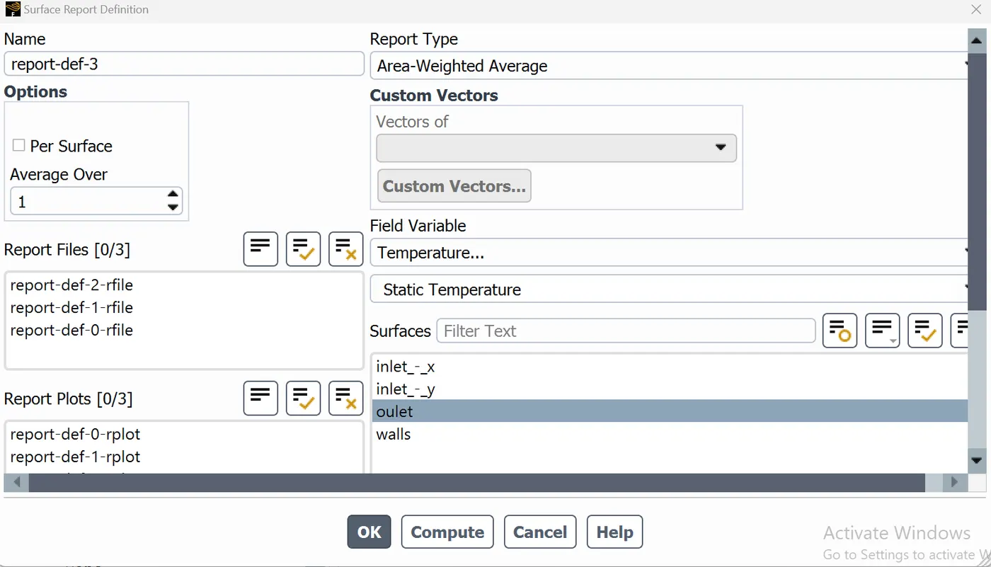
In order to attain the required graphs go to solutions under the solution window and choose definitions and under them choose area-weighted average and standard deviation graphs. Give temperature as fluid variable and outlet as surface. Give report file and report plot blue ticks.

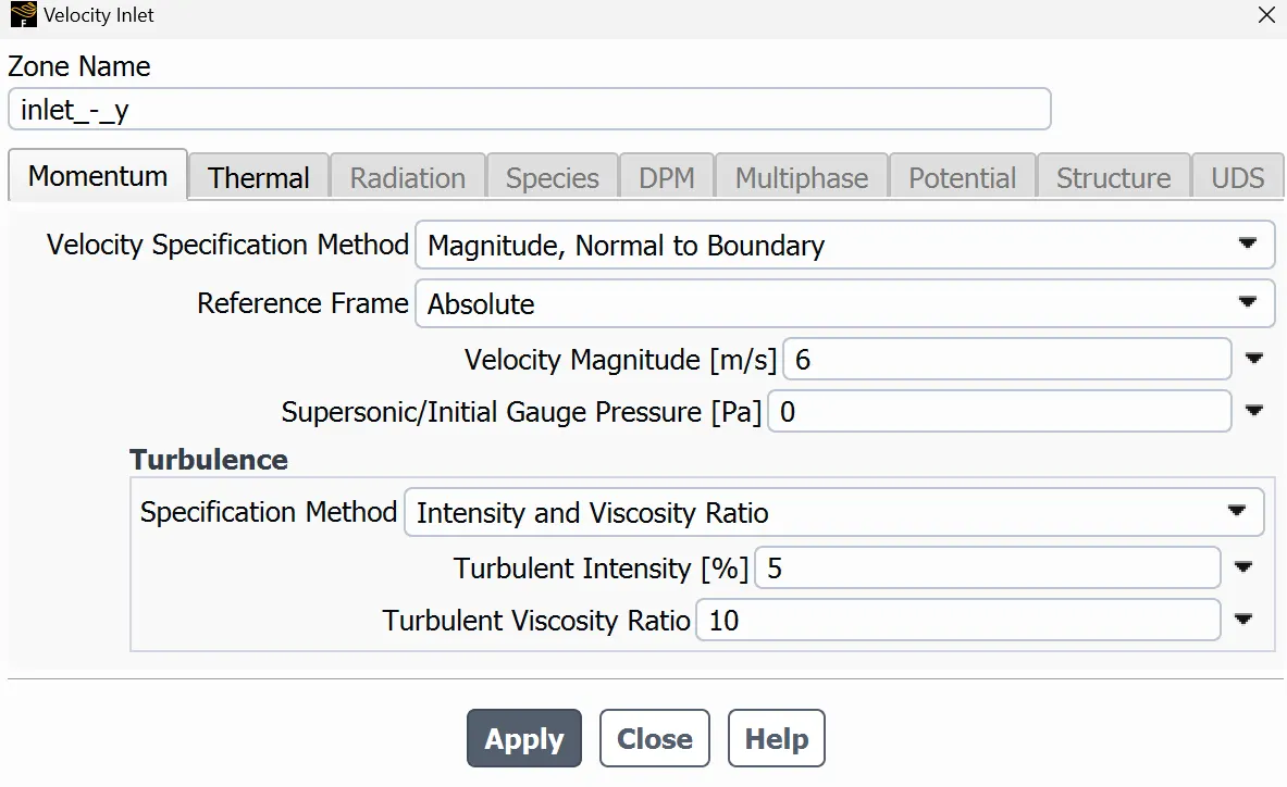
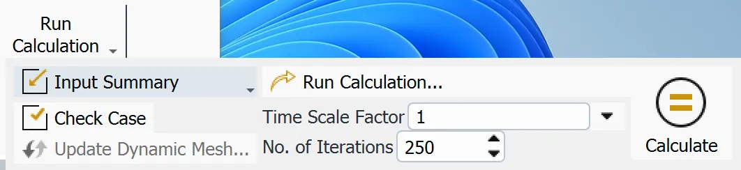
give initialization window as t =0 and run the iteration = 250 and calculate and so we obtain several graphs of residuals, standard deviation, and area-weighted average with respect to a number of iterations.

• Results

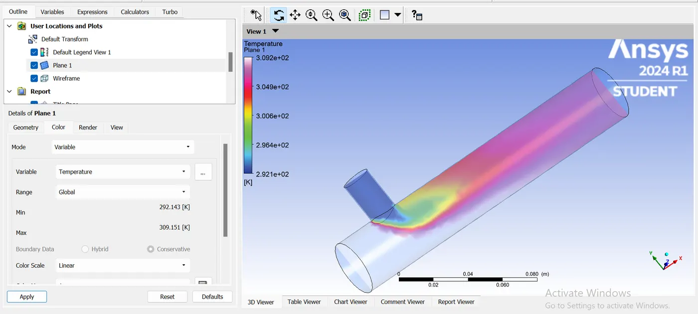
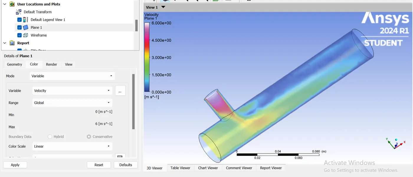
Hide the inlets and outlet and let's work on the walls to find the velocity and temperature distributions. Apply proper transparency for the walls. Insert the location plane onto the wall. Create the plane on xy plane with z value 0. Give proper transparency to the plane. Under temperature give the value of a variable as temperature.Give velocity also as the value as variable.

RESULTS

Case 1:

Considering the setup results of the short mixing tee with momentum ratio 2:

• Scaled Residuals

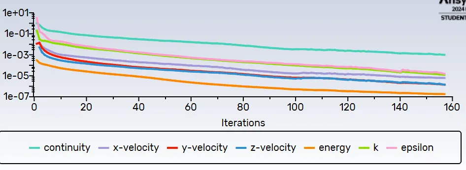
The total iterations over here was 161 which showed the different energy values plotted against the number of iterations. Continuity,x, y, and z velocities, energy, epsilon, and k values are found to decrease with the increase in the number of iterations(descending in ascending order).

• Report-def-0-rplot

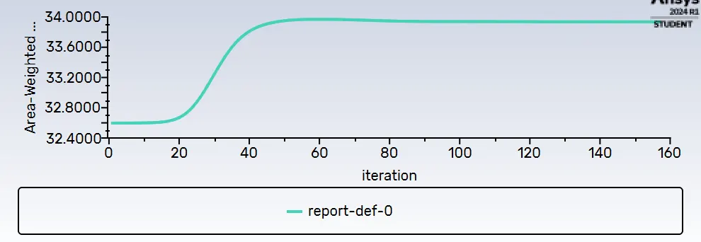
The area-weighted average is plotted against the iterations. The area-weighted average of value 32.6, after it reached 20 iterations, increased to a value of 34 at 40 iterations and went constant till the 161th iteration.

• Report-def-2-rplot

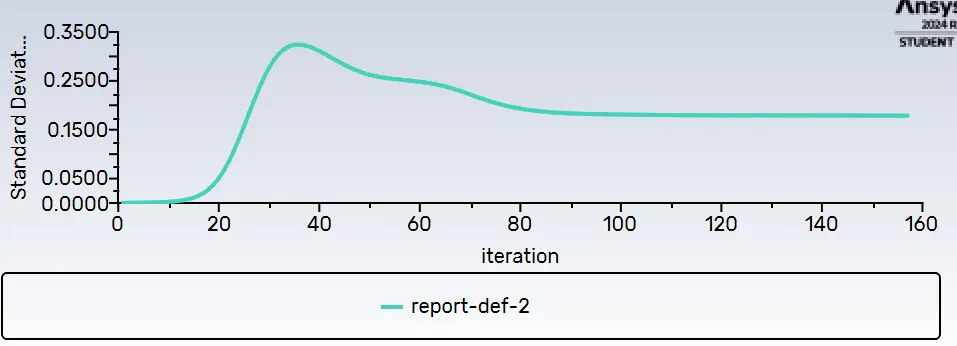
The standard deviation was plotted against the iterations. It shows that the value of standard deviation starts from 0 and is increased to a value of 39 before 50 iterations it goes almost constant throughout till the 161st iteration.

Considering the setup results of the short mixing tee with momentum ratio 4:

• Scaled Residuals

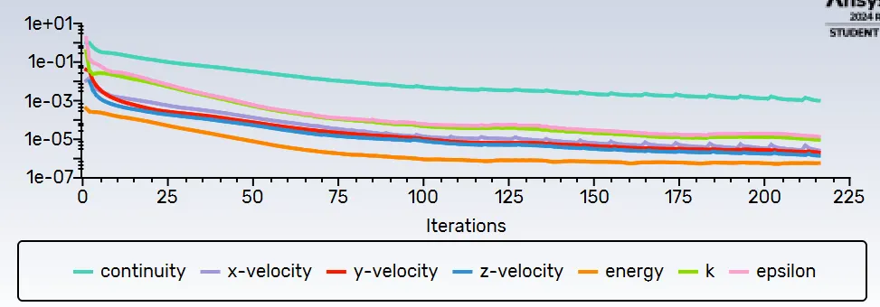
The total number of iterations over here was 216 which showed the different energy values plotted against the number of iterations. Continuity,x, y, and z velocities, energy, epsilon, and k values are found to decrease with the increase in the number of iterations.

• Report-def-0-rplot

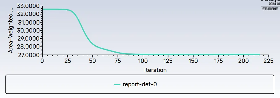
The area-weighted average is plotted against the iterations. The area-weighted average started at a value between 32.4 and 32.9 at the 0th iteration and it dropped after the 25th iteration from a value of 32.45, it goes almost constant from the 89th to 216th iteration to a value of 27.06.

• Report-def-2-rplot

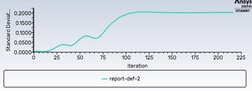
The standard deviation was plotted against the iterations. It shows that the value of standard deviation starts from 0.0059 to 0.2032 from iterations 2 to 116th and it goes almost constant throughout till the 216th iteration.

Considering the results of temperature and velocity of airflow through the mixing tee.For momentum ratio 2:

• Temperature

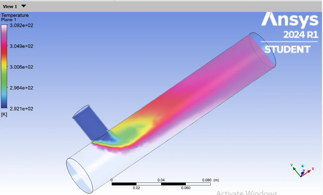
Considering the temperature of the flowing air into the mixing tee. The temperature is the lowest at the inlet - y (19 degrees C)and the most at the inlet -x(36 degrees C).

• Velocity

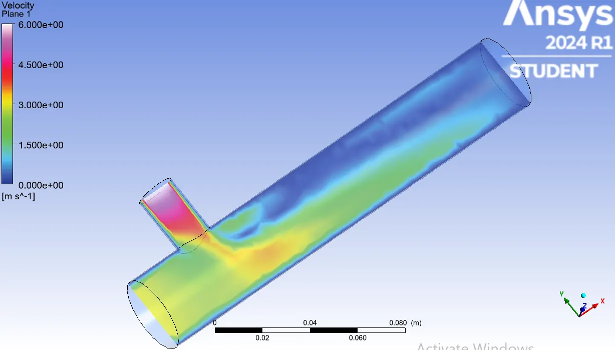
Considering the velocity of the flowing air into the mixing tee. The velocity is lowest at the inlet - x(3m/s) and the most at the inlet -y (6m/s).

Considering the results of temperature and velocity of airflow through the mixing tee.For momentum ratio 4:

• Temperature

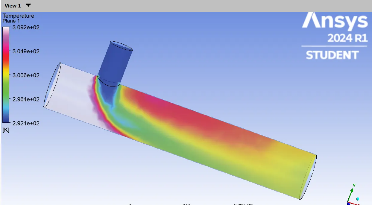
Considering the temperature of the flowing air into the mixing tee. The temperature is the lowest at the inlet - y (19 degrees C)and the most at the inlet -x(36 degrees C). The temperature at the outlet seems to be much cooler than in the case of the momentum ratio 2.

• Velocity

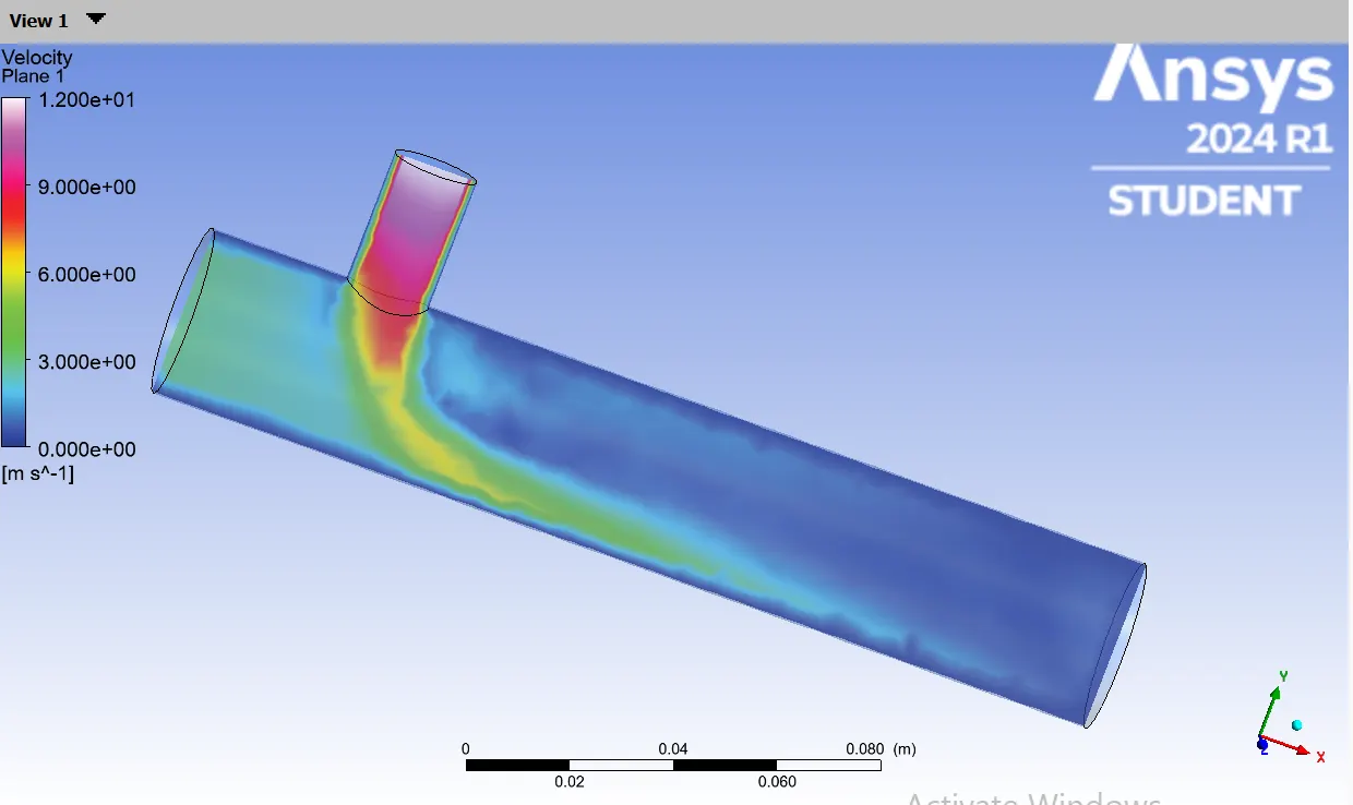
Considering the velocity of the flowing air into the mixing tee. The velocity is lowest at the inlet - x(3m/s) and the most at the inlet -y (12m/s). The velocity reaches 0 much faster than in the case of mentum ratio 2.

Case 2:

Considering the setup results of the long mixing tee with momentum ratio 2:

• Scaled Residuals

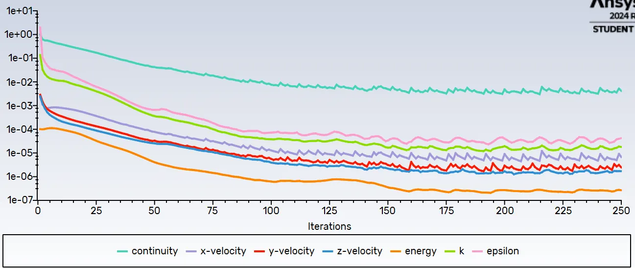
The total iterations over here was 250 which showed the different energy values plotted against the number of iterations. Continuity,x, y, and z velocities, energy, epsilon, and k values are found to decrease with the increase in the number of iterations.

• Report-def-0-rplot

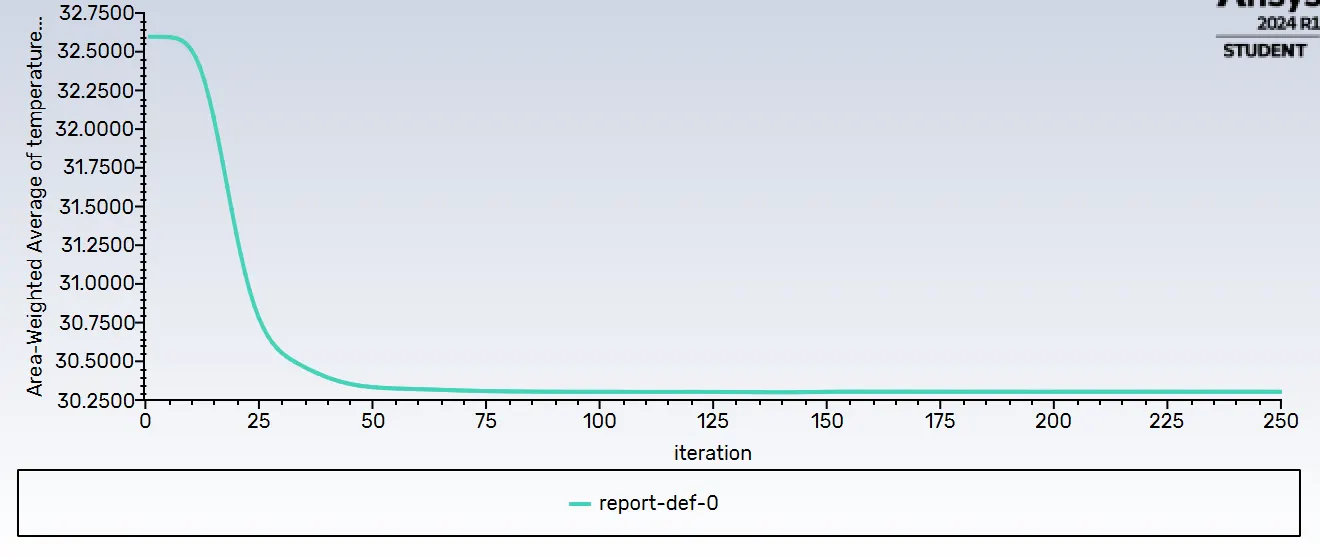
The area-weighted average is plotted against the iterations. The area-weighted average starts at a value 32.6 at 3rd iteration , after it reached 9th iteration,the value of area weighted average starts to drop from a value of 32.5 to 30 at 10 to 49 iterations and went constant till the 250th iteration.

• Report-def-2-rplot

The standard deviation was plotted against the iterations. It shows that the value of standard deviation starts from 0 and is increased to a value of 0.71 from 12 to 26 iterations,drops to 0.98 and it goes almost constant throughout till the 250 the iteration.

Considering the setup results of the short mixing tee with momentum ratio 4:

• Scaled Residuals

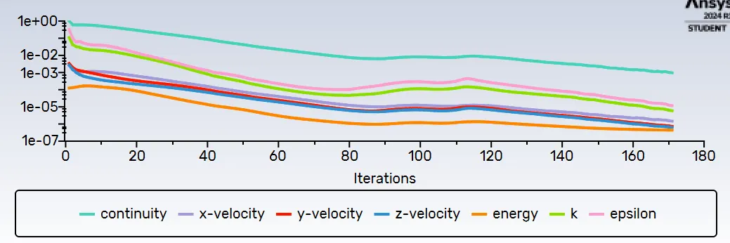
The total number of iterations over here was 171 which showed the different energy values plotted against the number of iterations. Continuity,x, y, and z velocities, energy, epsilon, and k values are found to decrease with the increase in the number of iterations.

• Report-def-0-rplot

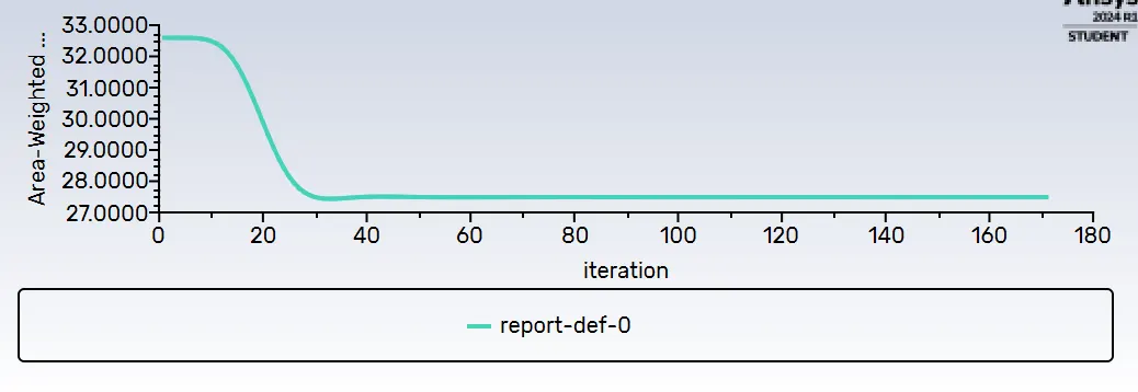
The area-weighted average is plotted against the iterations. The area-weighted average started at a value between 32.5 at the 2nd iteration and from 34.5 it drops to after the value of 27.4, it goes almost constant from the 32nd to 171st iteration to a value of 27.4.

• Report-def-2-rplot

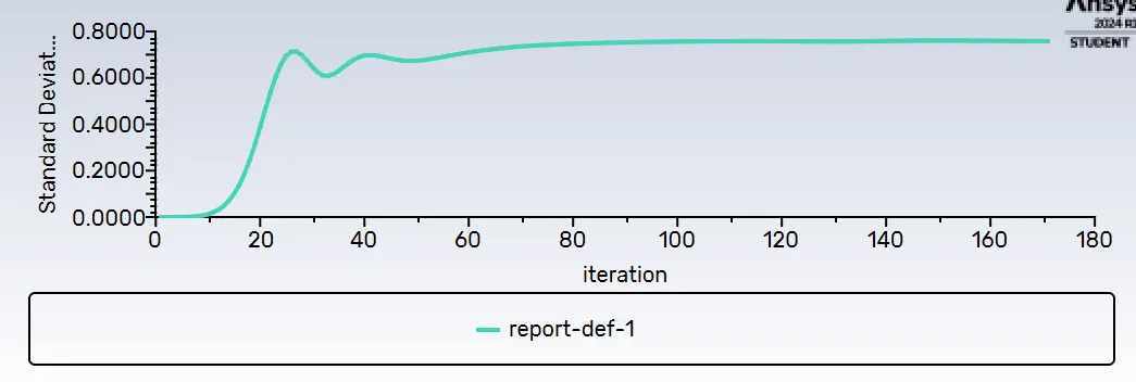
The standard deviation was plotted against the iterations. It shows that the value of standard deviation starts from 0 to 0.71 from iterations 0 to 25 and it goes almost constant throughout till the 171st iteration.

Considering the results of temperature and velocity of airflow through the mixing tee.For momentum ratio 2:

• Temperature

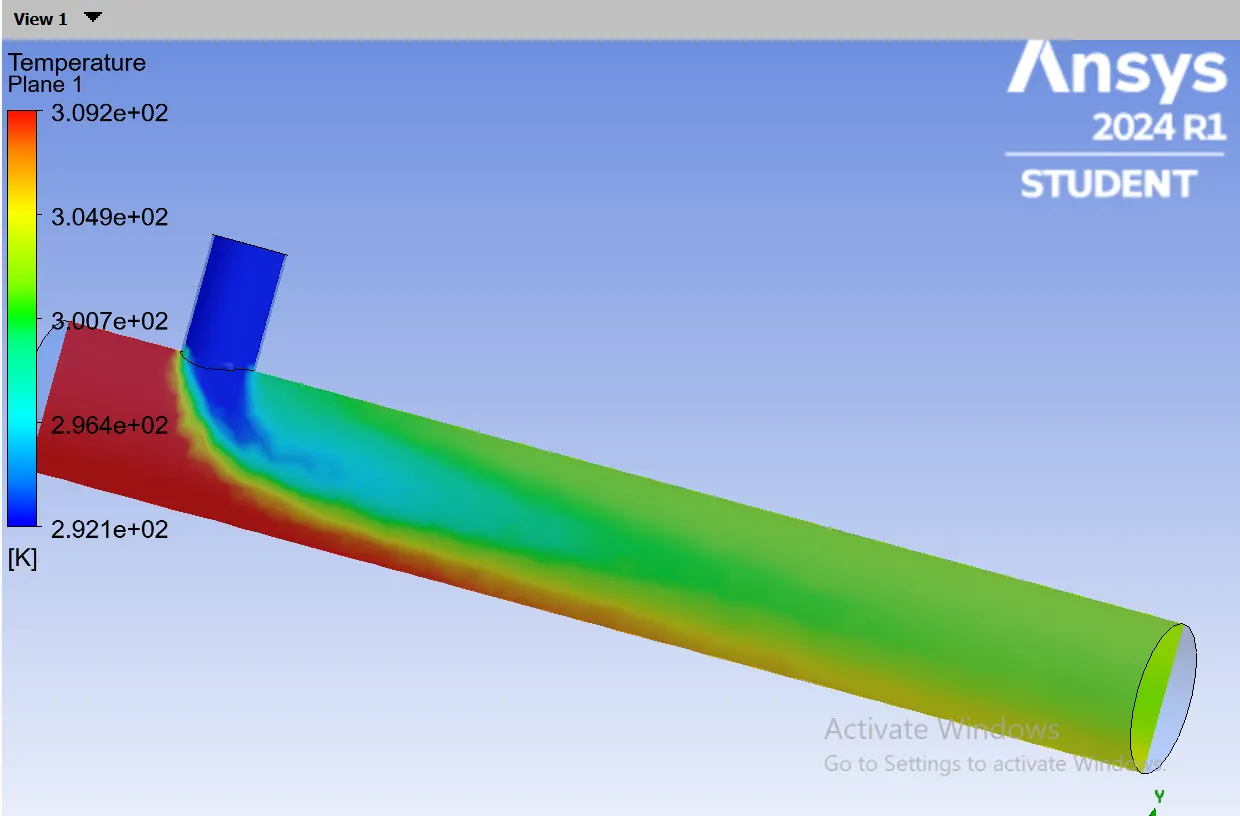
Considering the temperature of the flowing air into the mixing tee. The temperature is the lowest at the inlet - y (19 degrees C)and the most at the inlet -x(36 degrees C).

• Velocity

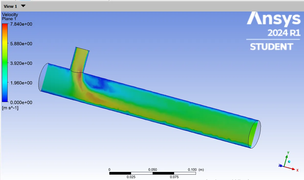
Considering the velocity of the flowing air into the mixing tee. The velocity is lowest at the inlet - x(3m/s) and the most at the inlet -y (6m/s).

Considering the results of temperature and velocity of airflow through the mixing tee.For momentum ratio 4:

• Temperature

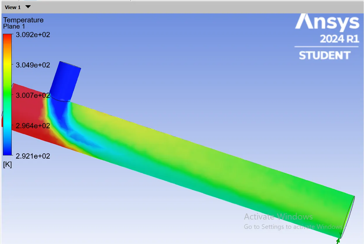
Considering the temperature of the flowing air into the mixing tee. The temperature is the lowest at the inlet - y (19 degrees C)and the most at the inlet -x(36 degrees C). The temperature at the outlet seems to be much cooler than in the case of the momentum ratio 2.

• Velocity

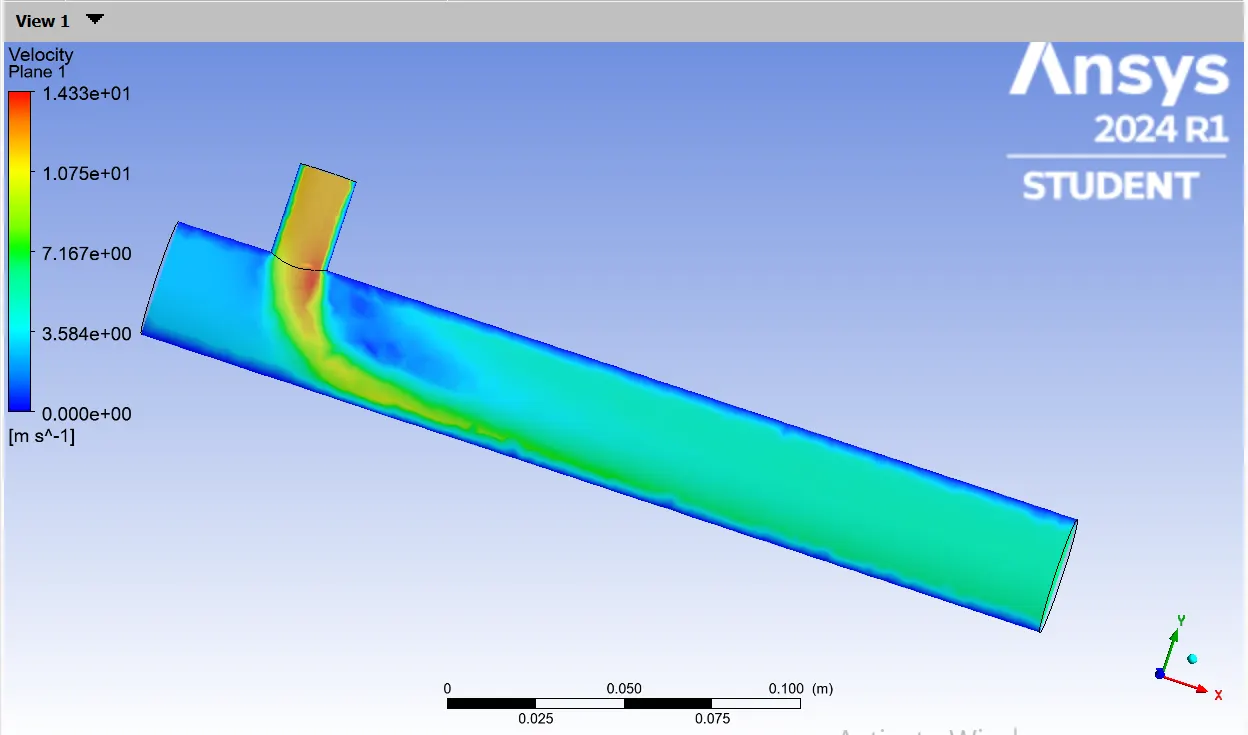
Considering the velocity of the flowing air into the mixing tee. The velocity is lowest at the inlet - x(3m/s) and the most at the inlet -y (12m/s). The velocity reaches 0 much faster than in the case of mentum ratio 2.

COMPARISON TABLE BETWEEN THE SHORT AND LONG MIXING TEES

	MIXING TEE SHORT - RATIO 2	MIXING TEE SHORT- RATIO 4	MIXING TEE LONG - RATIO 2	MIXING TEE LONG-RATIO 4
CELL COUNT	14400	14400	17992	17992
AVERAGE OUTLET TEMPERATURE	33.93 C 0.178 C standard deviation	27.061 C 0.237 C standard deviation	30.30 C 1.002 C standard deviation	27.48 C 0.758 C standard deviation
NUMBER OF ITERATIONS FOR CONVERGENCE	161	216	250	171

CONCLUSION

• K - epsilon converges faster and thus is also cheaper. But, both converge at some point and give similar results.
• The temperature drop is more when the momentum ratio is high. A possible cause is turbulent mixing.
• The numerical/computational solutions go hand in hand with analysis solutions.
• For best results, longer pipe lengths and higher momentum ratios can be preferred.