Week 1- Mixing Tee

Aim : Given Flow through mixing tee (i.e. short and long), set up steady-state simulations to compare the mixing effectiveness when hot inlet temperature is 36⁰C & the Cold inlet is at 19⁰C.

Use the k-epsilon and k-omega SST model for the first case and based on your judgment use the more suitable model for further cases. Giving the reason for choosing a suitable model is compulsory.

1. Case 1
   • Short mixing tee with a hot inlet velocity of 3m/s.
   • Momentum ratio of 2, 4.
2. Case 2
   • Long mixing tee with a hot inlet velocity of 3m/s.
   • Momentum ratio of 2, 4.

Momentum ratio = velocity at cold inlet / velocity at hot inlet

In a table, compare the following values from the 2 cases.

1. Cell count
2. Average outlet temperature
3. Number of iterations for convergence

To calculate:

1. Velocity and temperature contour plots on the cut planes along and across the pipe.
2. Velocity and temperature line plots along and across the length of the pipe.
3. Perform Mesh independent study for any one case.
4. Discuss the effect of length and momentum ratio on results.

Introduction:

T Joint is used as flow control devices where in mixing tee is used for mixing 2 flow streams at difference temperatures resulting in combined flow stream of desired temperature.

Applications: Air conditioning System

Scope: This challenge helps us in investigating the mixing effectiveness by varying the length of tee and velocity at which the two fluid enters. Momentum ratio is the ratio of inlet velocity of cold flow / inlet velocity of hot fluid.

Since the fluid mixing involves turbulence and to study the turbulence effect we use K-epsilon turbulence model where in we simulate the mean flow characteristics of the turbulent flow condition.

Relizable K- epsilon is used since it exhibits superior peformance when flow involves rotation and boundary layers with adverse pressure gradients. It is effective for predicting the flow behavior at region away from the wall.

Procedure:

1. Geometry preparation

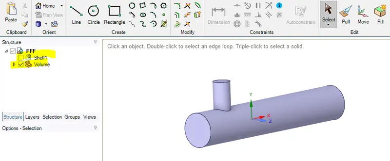
• IMPORT GEOMETRY IN SPACE CLAIM--> PREPARE --> VOLUME EXTRACTION --> SELECT EDGES --> CLICK TICK. THEN In STRUCTURE > MIXING TEE SHORT > UNSELECT SHELL1 --> SUPPRESS FOR PHYSICS --> CLOSE GEOMETRY

2. Mesh

• OPEN MESH -->ENTITY SELECTION > FACE SELECTION--> select the faces of the geometry to be mentioned as boundaries NAMELY INLET X,INLETY,OUTLET AND WALLS
• MESH -- > GENERATE MESH.
• Initailly keep the geometry in Y-direction. Now by using SECTION PLANE BUTTON, click and drag at the center to foam a line, so that it cuts the geometry.
• QUALITY --> MESH METRIC --> ELEMENT QUALITY --> C GRAPH ( AS LONG AS ELEMENT QUANTITY is not lower than 5%, SIMULAION RUNS)
• Close the Mesh

3. Set Up

• DOUBLE CLICK SETUP -- > FLUENT LAUNCHER -->DOUBLE PRECISION.
• Ansys Fluent is opened.
• In Graphics window --> GEOMETRY AND CONSOLE window is displayed.
• SETTING UP DOMAIN -->MESH --> select CHECK. Then in CONSOLE WINDOW --> it shows 'CHECKING MESH…. DONE'
• To Change the Units, SETTING UP DOMAIN --> click Units
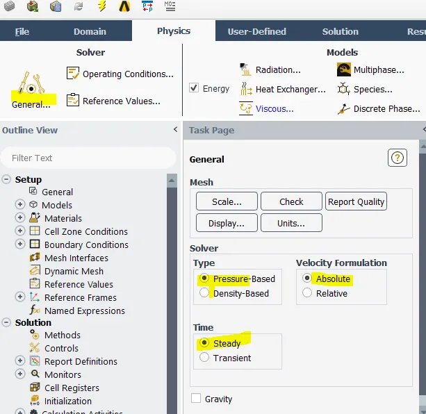
• SETTING UP PHYSICS --> SOLVER --> select Time = STEADY, Type = PRESSURE BASED & Velocity Formation = ABSOLUTE.

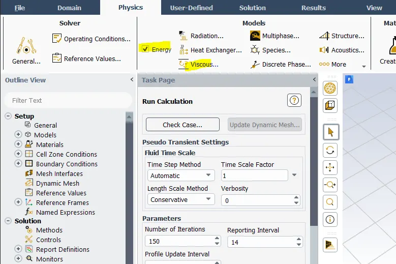
• SETTING UP PHYSICS --> MODELS > select ENERGY. VISCOUS MODEL --> Model --> K-epsilon Model, REALIZABLE K-epsilon Model, STANDARD WALL FUNCTIONS -->OK.

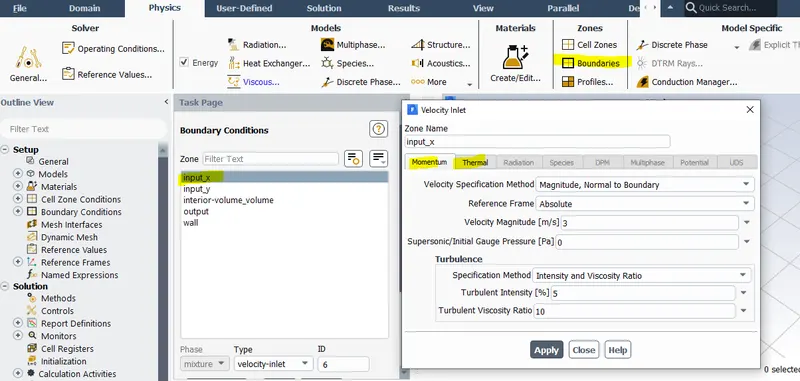
• SETTING UP PHYSICS-->BOUNDARIES -->ASK PAGE opens. Enter the values for Momentum, Thermal for both 'inlet-x' and 'inlet-y'. Then click OK.
• FOR BOUNDARY 'outlet', the GUAGE PRESSURE (PASCAL) = 0 is available by default > Click OK.

4. Solution

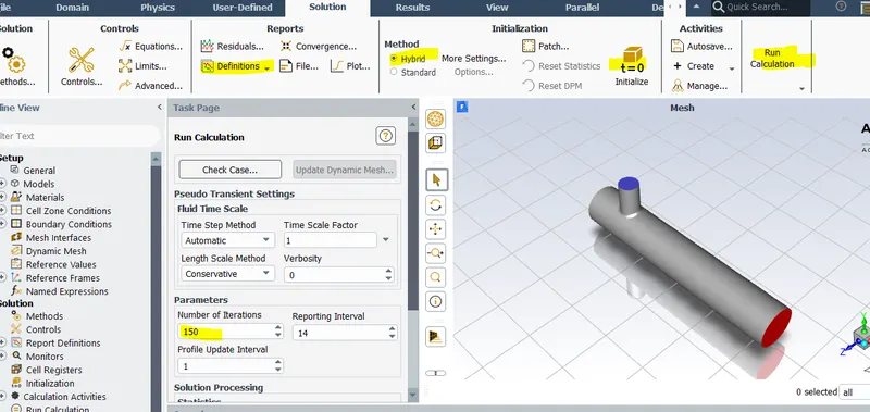
• SOLVING --> CONTROLS, REPORTS, INITIALIZATION, RUN CALCULATION.
• REPORTS-- > DEFINITIONS --> NEW --> SURFACE REPORT -->AREA WEIGHTED AVERAGE. Similarly, select STANDARD DEVIATION. For both the cases, a 'SURFACE REPORT DEFINITION WINDOW'pops up > select the FIELD VARIABLE = Temperature
• CREATE --> select REPORT FILE and REPORT PLOT.
• INITIALIZATION --> select METHOD = HYBRID --> click t=0 INITIALIZE
• RUN CALCULATION --> NO. OF ITERATIONS =150 and press CALCULATE.

5. Results and Discussion:

• Double click on RESULTS --> Post process window opens
• volume_volume --> select 'wall volume_volume' and hide all inlets and outlets
• Plane Creation --> Top Toolbar --> INSERT-- > LOCATION --> PLANE
• Plane 1 --> Double click --> COLOR --> Mode = VARIABLE-- > In VARIABLE --> select TEMPERATURE > Apply

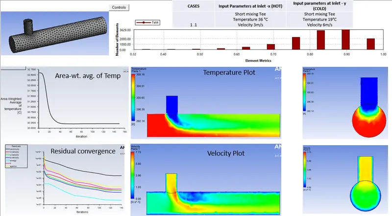
CASE1.1

CASE 1.2

CASE 2.1

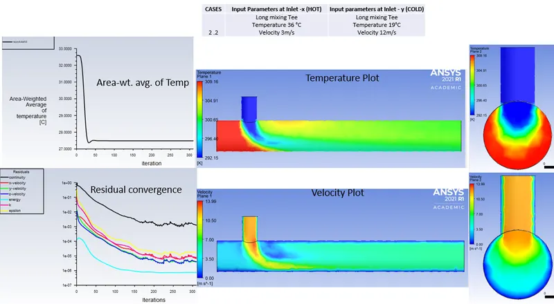
CASE 2.2

Summary

CASES	Input Paramters at Inlet -x (HOT)	Input parameters at Inlet - y (COLD)	Size of Element	Avg Outlet Temp (°C)	No. of iterations for Convergence	Std Deviation of Temp (°C)
1 .1	Short mixing Tee Temperature 36 °C Velocity 3m/s	Short mixing Tee Temperature 19°C Velocity 6m/s	12760	30°C	125	1.6
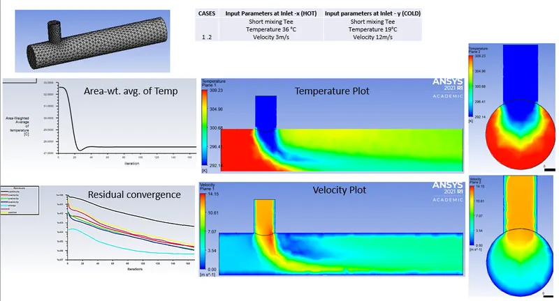
1 .2	Short mixing Tee Temperature 36 °C Velocity 3m/s	Short mixing Tee Temperature 19°C Velocity 12 m/s	12760	27.5°C	165	1.1
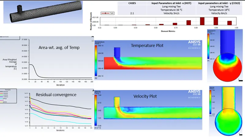
1 .3	Long mixing Tee Temperature 36 °C Velocity 3m/s	Long mixing Tee Temperature 19°C Velocity 6m/s	15689	30°C	190	1.4
1 .4	Long mixing Tee Temperature 36 °C Velocity 3m/s	Long mixing Tee Temperature 19°C Velocity 12 m/s	15689	27.5°C	260	0.55

Inference:

• Case 1.1 : It is envisaged from the table that non uniform temperature distribution at the outlet is observed. This may be due to uneven mixing of hot and cold air.
• Case 1.2 : It is envisaged from the table that when compared to Case 1.1 better distribution of temperature at outlet is observed. This is due to more turbulence at the mixing zone due to high velocity of cold air but still some amount of hot air exists due to uneven mixing of cold and hot air.
• Case 2.1 : It is envisaged from the table that compared to short tee the distribution of temperature is uniform at the outlet is observed mainly due to increased length aiding even mixing of hot and cold air
• Case 2.2 : It is envisaged from the table that compared to short tee and Case 2.1 long tee the distribution of temperature is uniform at the outlet is observed. This is due to increased length and more turbulence at the mixing zone due to high velocity of cold air
• Boundary layer formation is observed in all case near the walls due to given no slip condition
• Effect of length: Not much effect is observed on the outlet temperature by increasing the tee length since both the cases shows same outlet temperature value refer Case 1.1 and Case2.1.
• Effect of momentum ratio on results: momentum ratio is the ratio of cold air velocity to hot air velocity. Thus by increasing the cold air velocity by a factor of 2 results in reduced outlet temperature. Cases 1.2 and 1.4 clearly depicts reduced outlet temperature to 27.5°C compared to its counter case 30°C. This is due to turbulent mixing which is the primary mixing occurs due to higher velocity of the cold air then the secondary mixing happens due to diffusion.
• Primary mixing contributes more towards the outlet temperature.

CASES	Element Size	Size of Element	Avg Outlet Temp (°C)	No. of iterations for Convergence	Std Deviation of Temp (°C)
1.1	10.219e-003m	12760	30°C	125	1.6
1.1	5e-003 m	14420	30°C	145	1.25

Inference:

Grid size was reduced to check its effect on solution. Since the problem is simple the default grid size itself is sufficient to converge. There was no difference in outlet temperature observed even when grid size is reduced by 50 %. Thus the default grid size itself is sufficient and independent of solution.

CONCLUSION:

The steady state simulations to compare the mixing effectiveness when both hot inlet temperatures and cold inlet temperatures was successfully studied using Ansys Fluent. Signifcant change in outlet temperature is observed by varying the momentum ratio without changing the tee length.