Week 1- Mixing Tee

1. Case 1
• Short mixing tee with a hot inlet velocity of 3m/s.
• Momentum ratio of 2, 4.
2. Case 2
• Long mixing tee with a hot inlet velocity of 3m/s.
• Momentum ratio of 2, 4.

INTRODUCTION:

The function of mixing Tee is to provide proper mixing of quantities to get the desired result at the outlet.

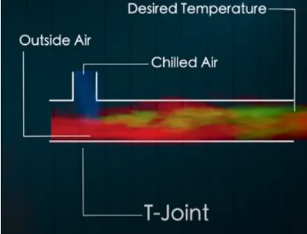
By controlling the velocity of chilled air we can get the desired temperature in the room.

ANSYS WORKFLOW:

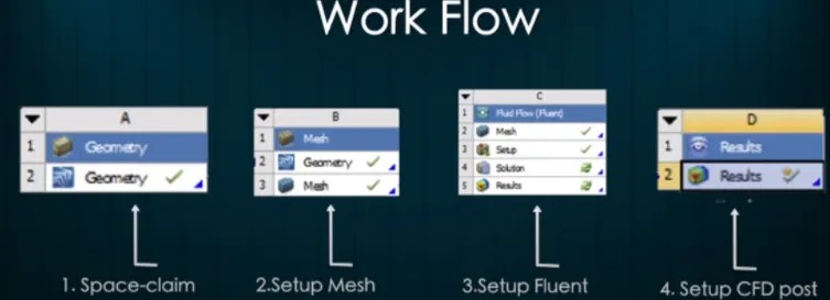
GEOMETRY: Construct a two or three dimensional representation of the object to be modelled and tested using the work plane coordinate system within ANSYS.

MESH: At this point ANSYS understands the makeup of the part. Now define how the modelled system should be broken down into finite pieces.

SETUP: The case setup will be done using ansys fluent

SOLUTION: Ansys fluent where run time result visualization is done

RESULTS: Post processing of results will be done here using CFD-post

SHORT TEE:

GEOMETRY SETUP:

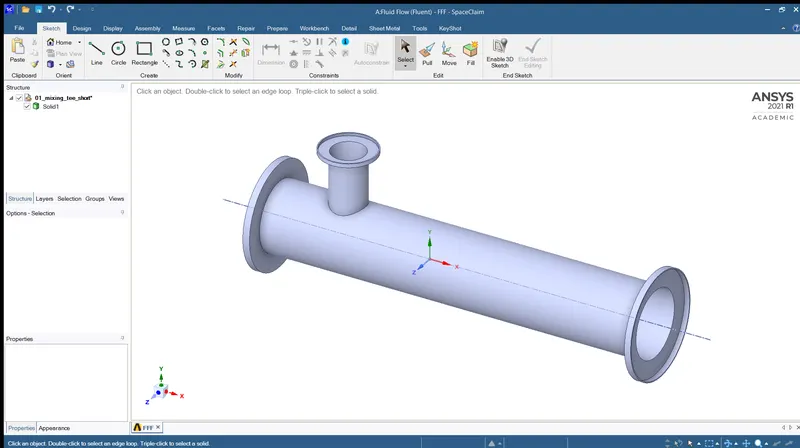
The computational models are uploaded to the Ansys Space Claim as a step file.

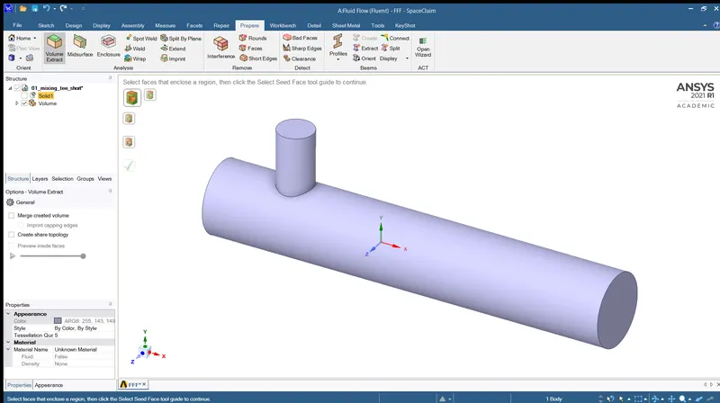
In this project, we are interested in performing fluid flow analysis through the geometry, hence we used the volume extraction option to extract the fluid volume from the geometry. Then the solid model is suppressed for physics from the fluid model to create mesh at the interested region.

MESH GENERATION:

The boundary names inlet_x, inlet_y, outlet and wall are defined using the named selection option.

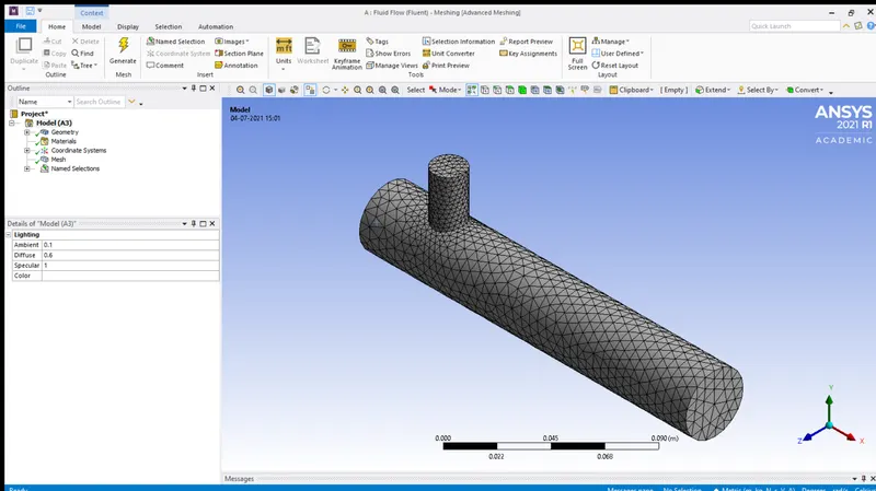
After generating the mesh, the number of nodes and elements are investigated using the statistics option. Then the mesh quality is checked by choosing the mesh metrices option in quality section.

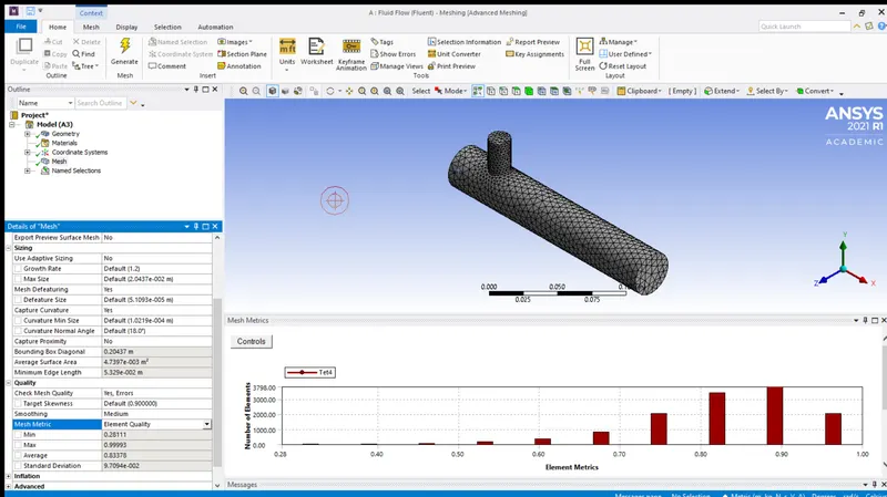
The element quality should not be less than 5%. In our case minimum mesh quality is 30%, so we can move ahead.

SETUP AND SOLUTION:

CASE 1:

• Short mixing Tee with a hot inlet velocity of 3m/s
• Momentum ratio of 2,4

CASE 1.1:

• Short mixing Tee with a hot inlet velocity of 3m/s
• Momentum ratio of 2

SETUPS	SHORT TEE (MR=2 AND HOT INLET VELOCITY = 3m/s)
	K-EPSILON	K-OMEGA
SOLVER TYPE	Pressure based	Pressure based
VELOCITY FORMULATION	Absolute	Absolute
TIME	Steady	Steady
VISCOUS MODEL	Realizable K-epsilon with standard wall function	K-omega SST model
MATERIAL	Air	Air
CELL ZONES	Fluid type : air	Fluid type : air
BOUNDARIES	· Inlet_x (velocity inlet) Velocity magnitude 3m/s Temperature - 360c · Inlet_y (velocity inlet) Velocity magnitude 6m/s Temperature – 190c · Outlet (pressure outlet) Gauge pressure – 0 pa · Walls – stationary walls	· Inlet_x (velocity inlet) Velocity magnitude 3m/s Temperature - 360c · Inlet_y (velocity inlet) Velocity magnitude 6m/s Temperature – 190c · Outlet (pressure outlet) Gauge pressure – 0 pa · Walls – stationary walls

The hybrid scheme is used for initialization and the no. of iterations are setup and then click on calculate option.

RESULTS:

K-EPSILON MODEL:

RESIDUAL PLOT:

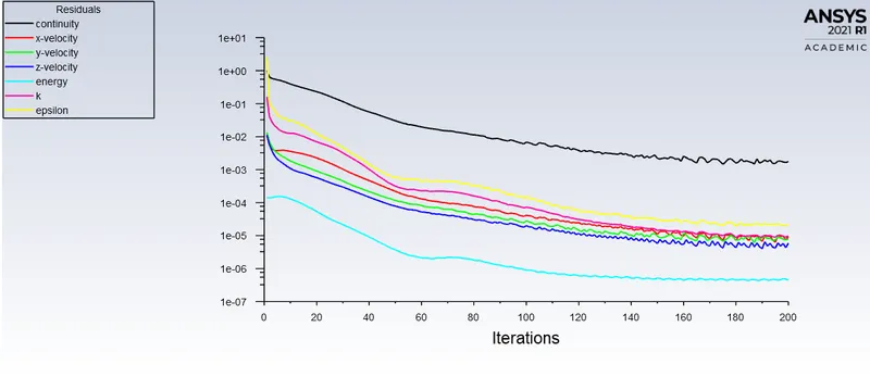
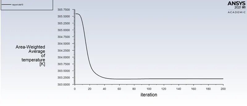
AREA WEIGHTED AVERAGE:

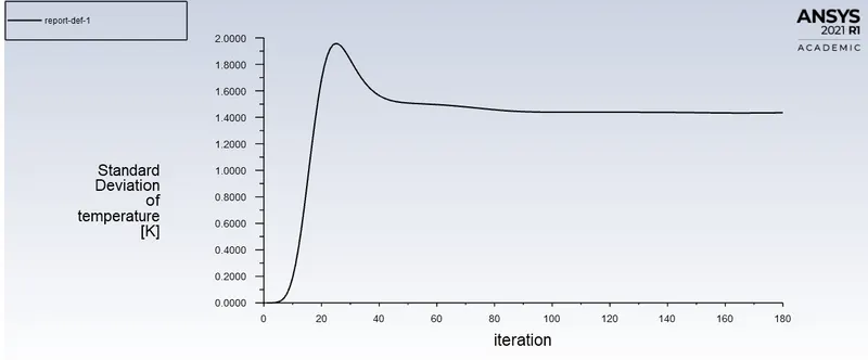
STANDARD DEVIATION:

CONTOUR PLOT:

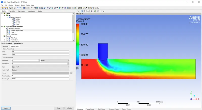
TEMPERATURE CONTOUR:

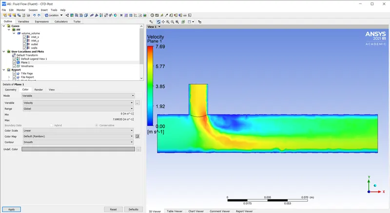
VELOCITY CONTOUR:

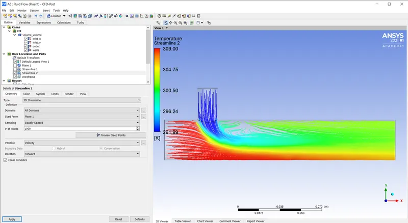
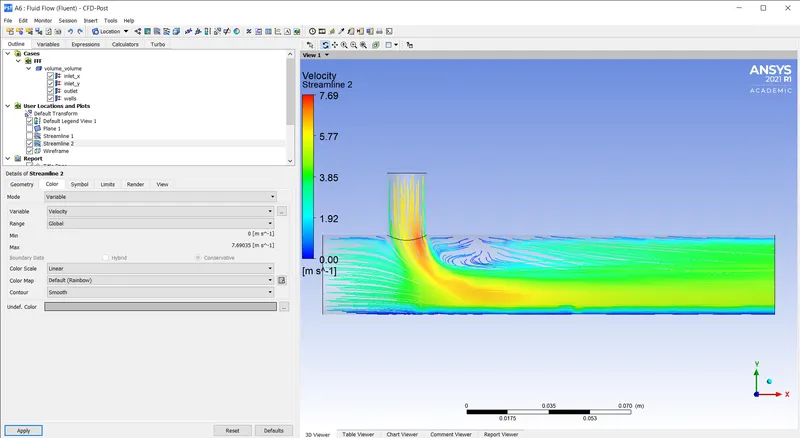
STREAMLINE PLOT:

TEMPERATURE:

VELOCITY:

K-OMEGA MODEL:

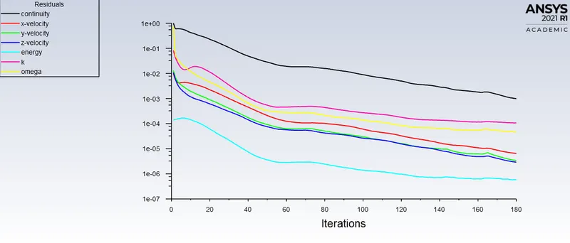
RESIDUAL PLOT:

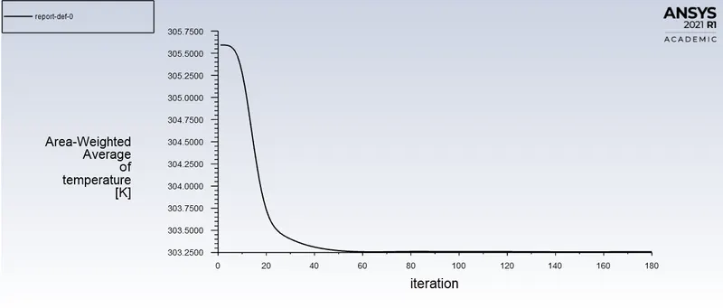
AREA WEIGHTED AVERAGE:

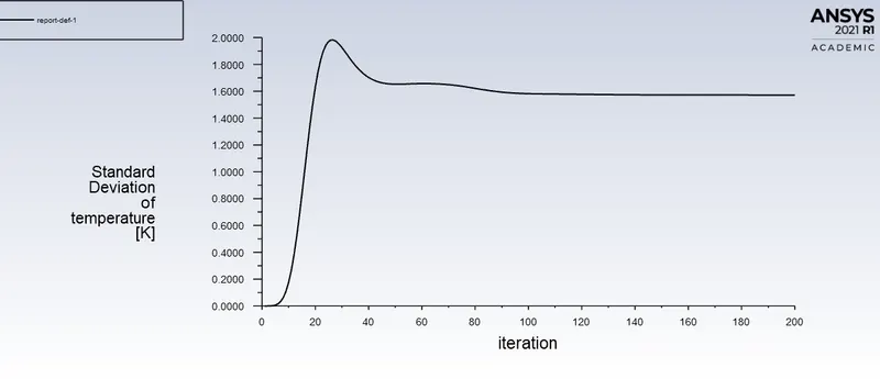
STANDARD DEVIATION:

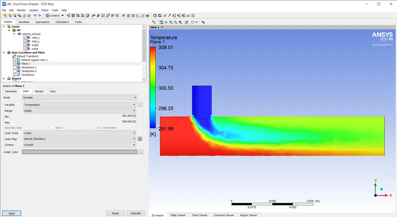
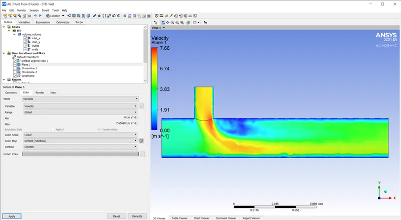
CONTOUR PLOT:

TEMPERATURE CONTOUR:

VELOCITY CONTOUR:

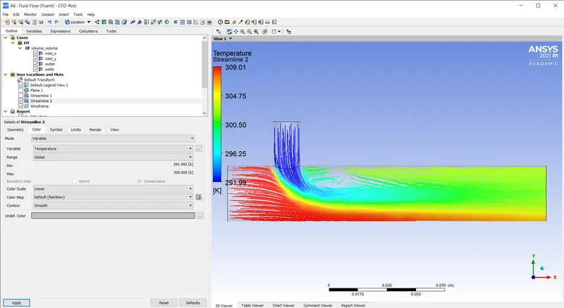
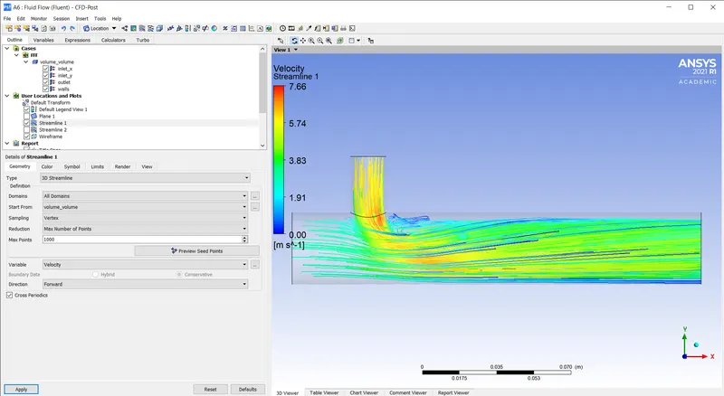
STREAMLINE PLOT:

TEMPERATURE:

VELOCITY:

SUMMARY:

	SHORT TEE (MR = 2)
	K-EPSILON	K-OMEGA
AVERAGE OUTLET TEMPERATURE [K]	303.413	303.458
STANDARD DEVIATION	1.5	1.6
NO OF ITERATIONS	150	170

CASE 1.2:

• Short mixing Tee with a hot inlet velocity of 3m/s
• Momentum ratio of 4

SETUPS	SHORT TEE (MR=2 AND HOT INLET VELOCITY = 3m/s)
	K-EPSILON	K-OMEGA
SOLVER TYPE	Pressure based	Pressure based
VELOCITY FORMULATION	Absolute	Absolute
TIME	Steady	Steady
VISCOUS MODEL	Realizable K-epsilon with standard wall function	K-omega SST model
MATERIAL	Air	Air
CELL ZONES	Fluid type : air	Fluid type : air
BOUNDARIES	· Inlet_x (velocity inlet) Velocity magnitude 3m/s Temperature - 360c · Inlet_y (velocity inlet) Velocity magnitude 12m/s Temperature – 190c · Outlet (pressure outlet) Gauge pressure – 0 pa · Walls – stationary walls	· Inlet_x (velocity inlet) Velocity magnitude 3m/s Temperature - 360c · Inlet_y (velocity inlet) Velocity magnitude 12m/s Temperature – 190c · Outlet (pressure outlet) Gauge pressure – 0 pa · Walls – stationary walls

The hybrid scheme is used for initialization and the no. of iterations are setup and then click on calculate option.

RESULTS:

K-EPSILON MODEL:

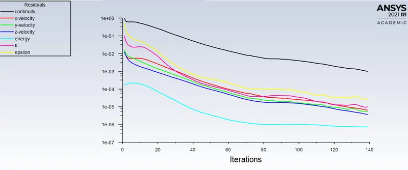
RESIDUAL PLOT:

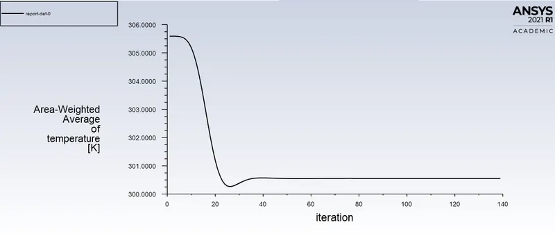
AREA WEIGHTED AVERAGE:

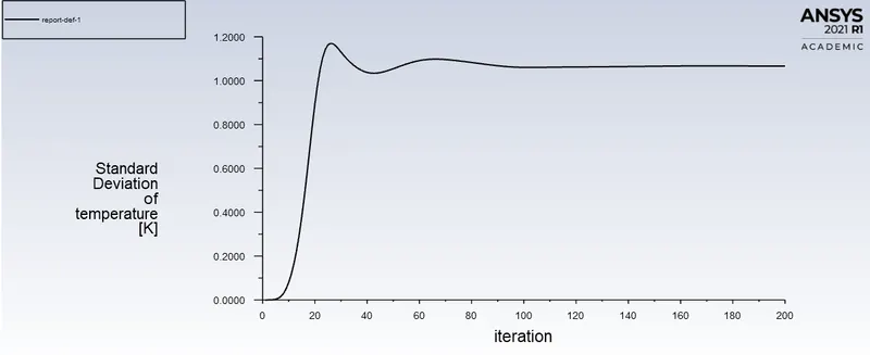
STANDARD DEVIATION:

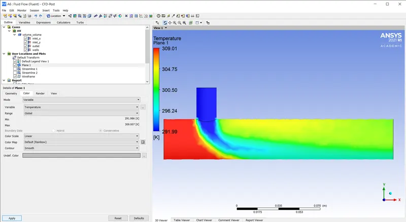
CONTOUR PLOT:

TEMPERATURE CONTOUR:

VELOCITY CONTOUR:

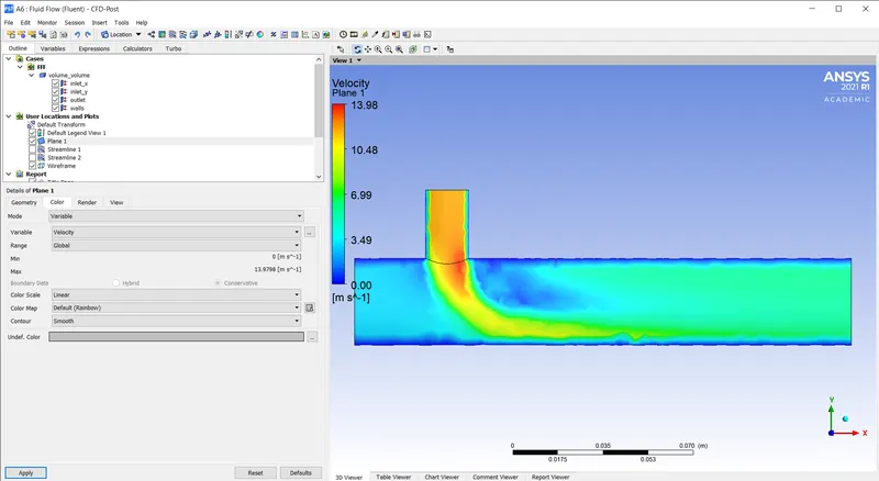
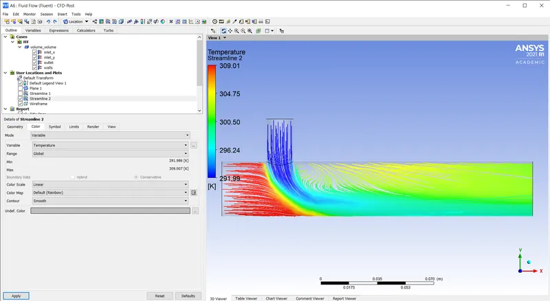
STREAMLINE PLOT:

TEMPERATURE:

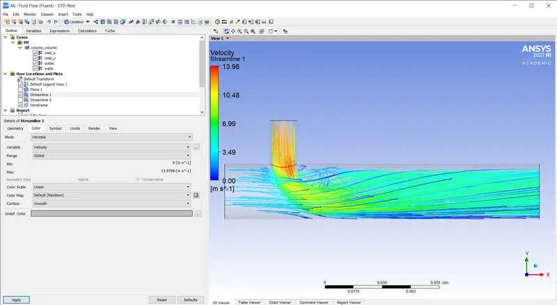
VELOCITY:

K-OMEGA MODEL:

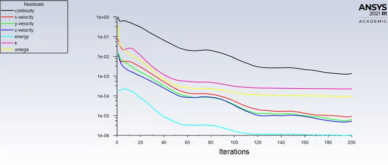
RESIDUAL PLOT:

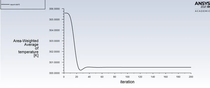
AREA WEIGHTED AVERAGE:

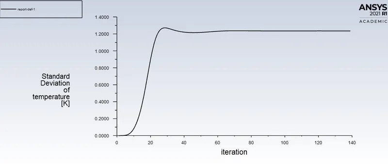
STANDARD DEVIATION:

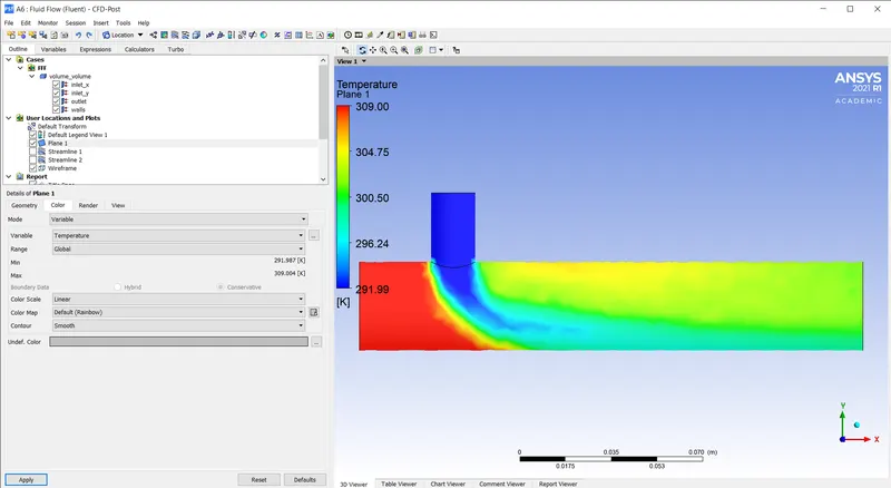
CONTOUR PLOT:

TEMPERATURE CONTOUR:

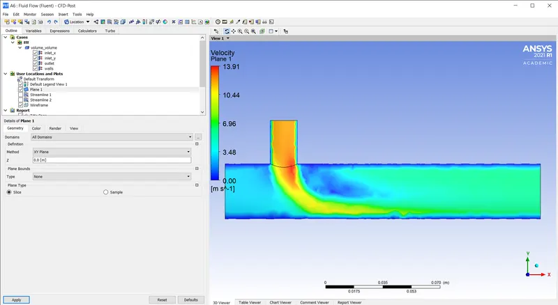
VELOCITY CONTOUR:

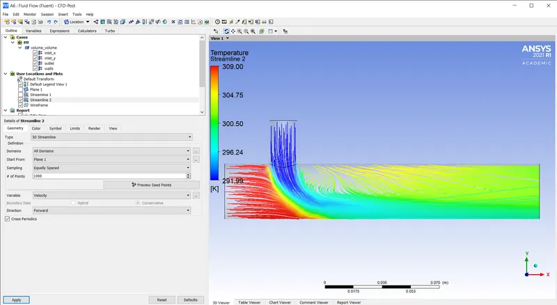
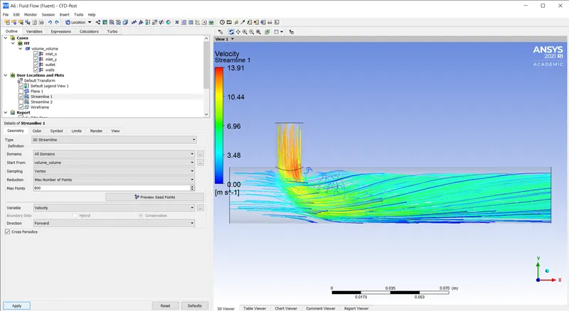
STREAMLINE PLOT:

TEMPERATURE:

VELOCITY:

SUMMARY:

	SHORT TEE (MR = 4)
	K-EPSILON	K-OMEGA
AVERAGE OUTLET TEMPERATURE [K]	300.396	300.38
STANDARD DEVIATION	1.1	1.2
NO OF ITERATIONS	130	160

ANALYTICAL SOLUTION:

MOMENTUM RATIO 2:

• Mass of hot fluid (m_h) = rho*a*V_h = 997*0.0009*3 = 2.69 kg/s
• Mass of cold fluid (m_c) = rho*a*V_c = 997*0.0009*6 = 1.35 kg/s
• Temperature of mixture (T_mixture) = (m_h*T_h + m_c*T_c)/(m_c + m_h) = 30.319⁰c = 303.319k

MOMENTUM RATIO 4:

• Mass of hot fluid (m_h) = rho*a*V_h = 997*0.0009*3 = 2.69 kg/s
• Mass of cold fluid (m_c) = rho*a*V_c = 997*0.0009*12 = 2.3928 kg/s
• Temperature of mixture (T_mixture) = (m_h*T_h + m_c*T_c)/(m_c + m_h) = 27.99⁰c = 300.99k

CONCLUSION:

AVERAGE OUTLET TEMPERATURE:

On comparing the both models with analytical solution we got nearly the same results.

ITERATIONS TO CONVERGE:

No. of iterations taken to converge is less for Realisable K-epsilon model than K-omega SST model.

STANDARD DEVIATION:

The standard deviation of k-epsilon model is less than k-omega model which shows the better mixing efficiency in k-epsilon model.

So based on the above observations the K-epsilon turbulence model is predicting the results accurately in less no. of iterations. So we can use realisable k-epsilon model for case 2