Week 1- Mixing Tee

AIM:

to set up steady-state simulations to compare the mixing effectiveness when hot inlet temperature is 36⁰C & the Cold inlet is at 19⁰C. Use the k-epsilon and k-omega SST model for the first case and based on your judgment use the more suitable model for further cases. Giving the reason for choosing a suitable model is compulsory.

1. Case 1
• Short mixing tee with a hot inlet velocity of 3m/s.
• Momentum ratio of 2, 4.
2. Case 2
• Long mixing tee with a hot inlet velocity of 3m/s.
• Momentum ratio of 2, 4.

in a table, compare the following values from the 2 cases.

1. Cell count
2. Average outlet temperature
3. Number of iterations for convergence

Introduction

Theory:

In this challenge we have to analyse the mixing of hot and cold air flow by using the geometry of tee pipe in which the flow is steady state and our flowing fluid is air, and also we have to see that how the fluid behaviour changes by change of length and momentum of ratio, we use some basic knowledge of CFD in this challenge and use the Ansys fluent to solve the challenge. In challenge we get to learn how the boundary condition plays role in challenge, and how velocity and temperature changes with change lengths and air flow

Modelling Approach:

1.Pre-processing:

Discussing the modelling approach, we first pre-process the geometry in space claim we open the geometry in space claim and then we remove the unwanted parts and edges only takes basic geometry then we close the space claim. Then moving to next step we open meshing module in which we name the different inlets and different outlets and walls first. Then we cut the section from half w.r.t xy axis so we can provide healthy mesh to model and moving to next step we provide mesh in meshing section in which we select element size as 0.0015 then we close the meshing module

2.Processing:

In processing we open the fluent in which we first check in the box of energy as it is related to temperature, then we select the model based on accuracy of result and convergence. then we add material or fluid which going to flow through pipe inn which we select air as fluid. Then we check the boundary conditions which we define in pre-processing like inlet-x, inlet-y, outlet, walls. While defining this condition we set the velocity and temperature values there. Then we select the residuals plot we want. Then we initialize the value then we run the calculation and we get those data. After getting iterations the processing ends in this stage if result gets converged then iterations stops automatically. And popup comes as solution converged. Here influent we can get the values we want by just playing with those keys

3.post-processing:

In post processing we opens the post cfd where we gets the results of our cfd model we get here contour , line plots here we get those velocity line plot, temperature line plot, contour temp plot, contour velocity plot etc by just adding the line and plain in between the pipe and on that plane we get the data like how temp flows and velocity flows

Results:

model selected between k-epsilon and k-omega and reason behind its selection

1. To choose the most preferable model between k-epsilon and k-omega we use the equation given in problem in which we calculate the t-mixture which we get the 30.25 C something and in k-epsilon we get that value of 30.30C and for k-omega we get 30.50C hence both are close to our check equation value.
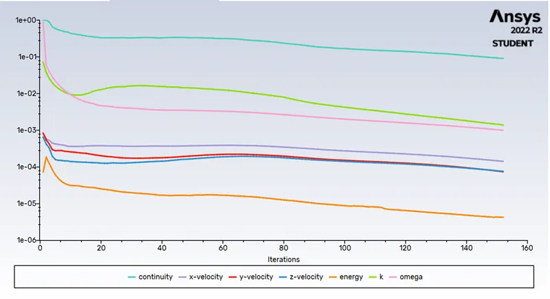
2. But when we carry out the iteration by setting the number of iteration value as 1000 the k-epsilon complete all the iteration and still not converged whereas the k-omega takes only 150 iterations to converged so by this conversion reason we use the k-omega for further case and calculations.
3. Third and most important reason to select the k-omega model over k-epsilon is the condition suited to y+ >30 value or the model more suited to this condition and our maximum y+ value here is 20 and as we see the k-epsilon only valid for turbulent flow and non-separatable flow and also have stability issues due to numerical stiffness, whereas k-omega model is essentially a Reynolds number model and use to resolve a mesh y+<1.

Case 1 short tee mixing plots and graphs

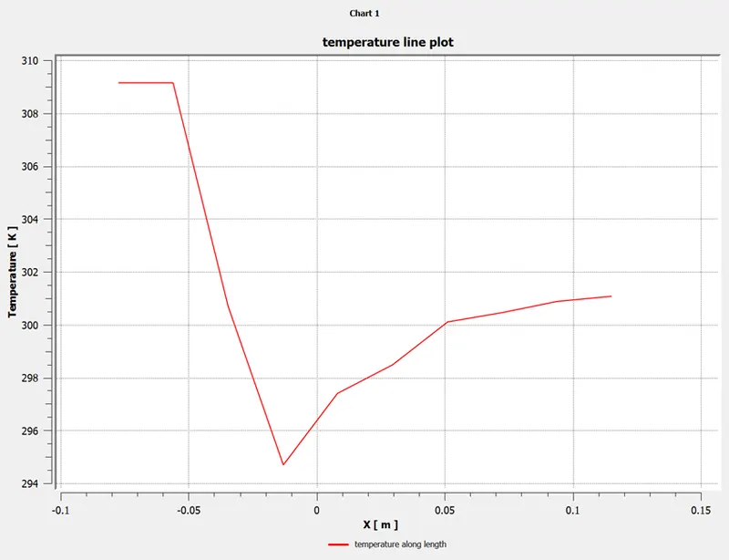
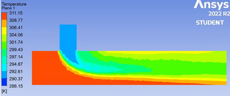
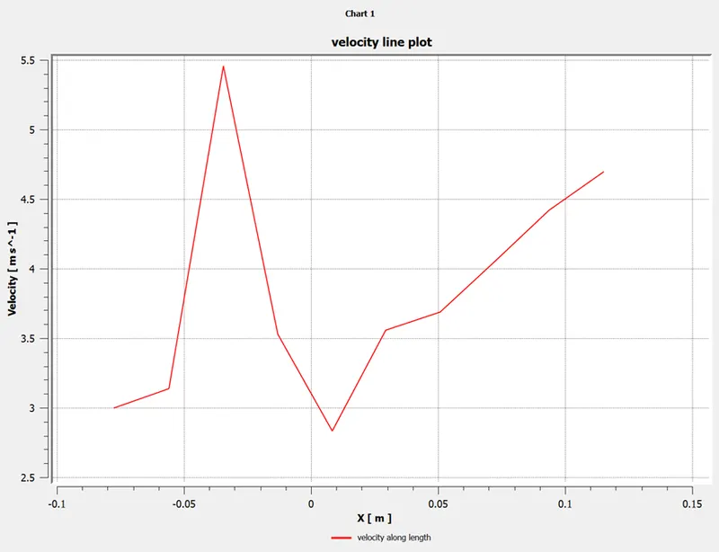
plots are given below for the case 1 with momentum ratio 2

Plot 1. Scaled residuals convergence plot(case 1, momentum ratio 2

Plot 2. Temperature line plot along length (case 1, momentum ratio 2)

Plot 3. Temperature Contour plot (case 1 , momentum ratio 2)

Plot 4. Velocity line plot (case 1, momentum ratio 2)

Plot 5. Velocity contour plot (case 1, momentum 2)

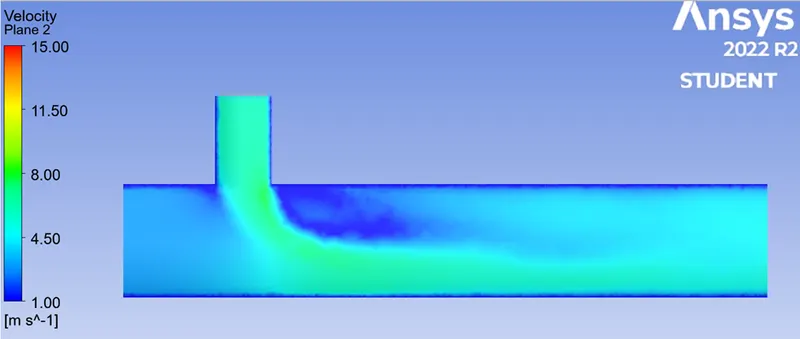
Short Tee mixing with momentum ratio of 4 :

As we see the plots of momentum 2 in short tee above now we goanna see the plots and graphs we get when we take momentum 4

Plot 6. Scaled residual convergence plot for short tee, momentum ratio 4

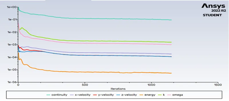
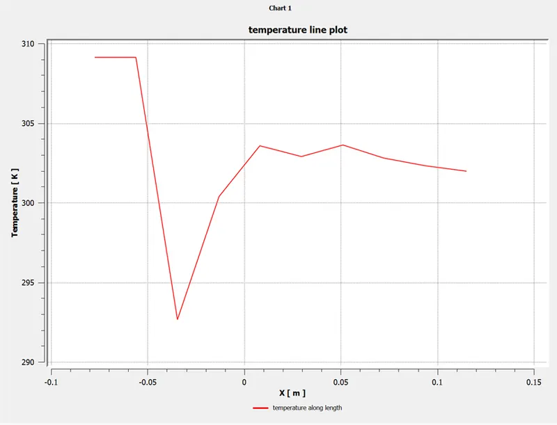
Plot 7. Temperature line plot case 1 momentum 4

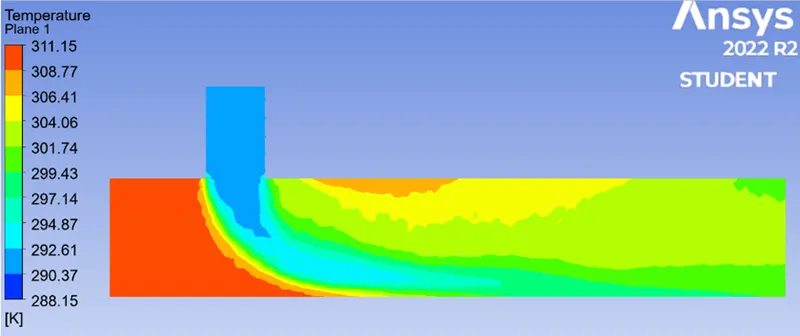
Plot 8. Temperature contour plot case 1 momentum 4

Plot 9. Velocity line plot case 1, momentum 4

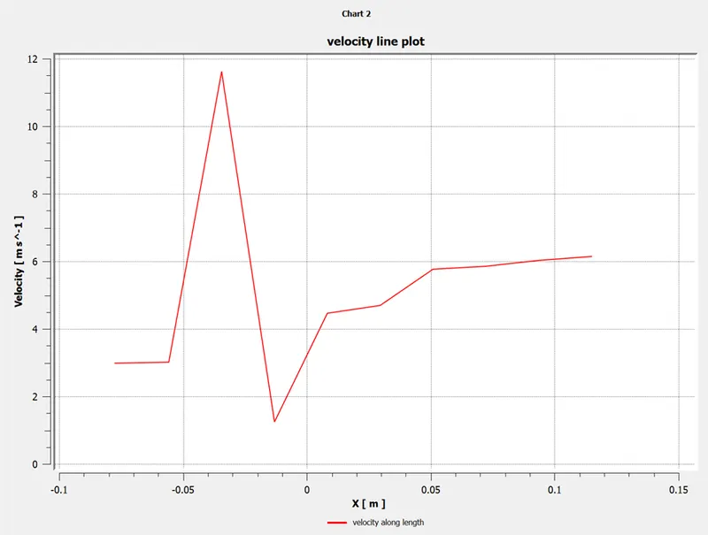
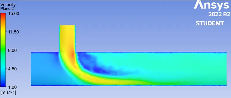
Plot 10. Velocity contour plot case 1 momentum 4

Case 2 long tee mixing :

Plots Long tee with Momentum ratio of 2

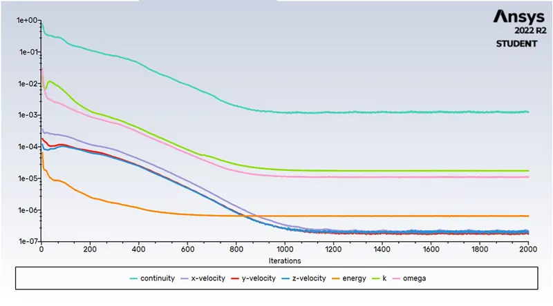
Plot 11. Scaled residuals convergence plots of long tee momentum ratio 2

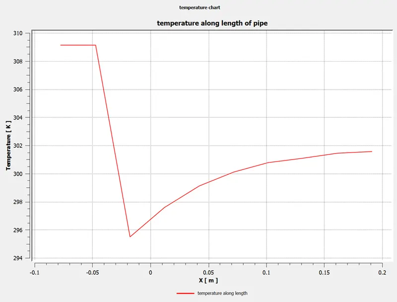
Plot 12. Temperature line plot long tee momentum ratio 2

Plot 13. Temperature Contour plot long tee momentum ratio 2

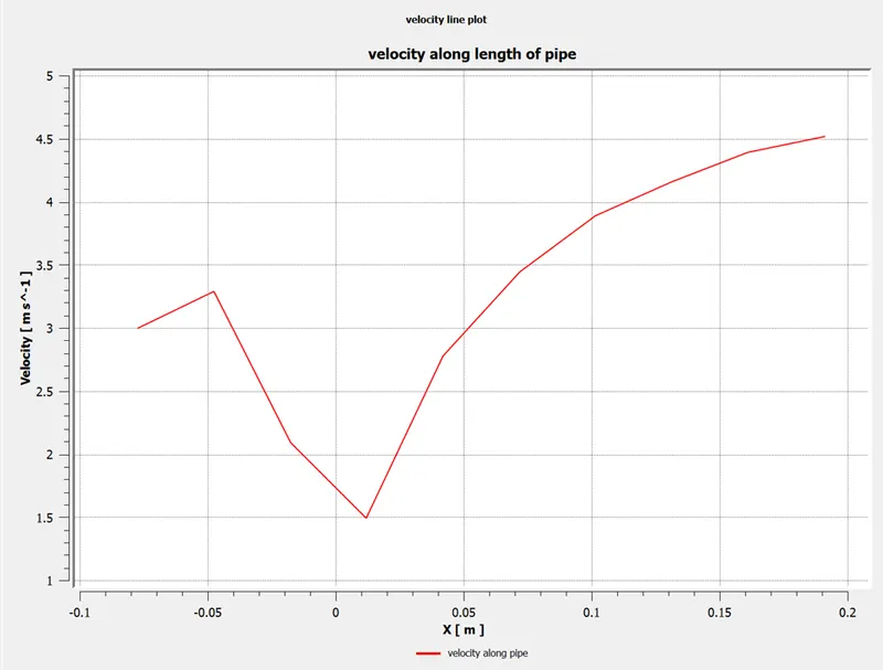
Plot 14. Velocity line plot long tee momentum ratio 4

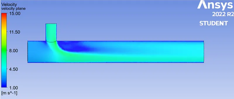
Plot 15. Velocity contour plot long tee momentum ratio 4

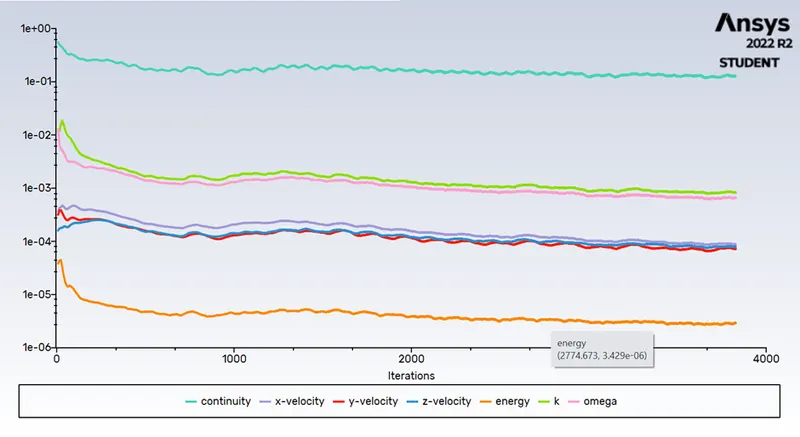
Long tee with momentum ratio 4 :

Plots

Plot 16. Scaled residuals convergence plots

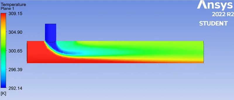
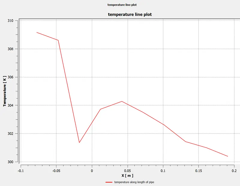
Plot 17. Temperature line plot along the pipe long tee momentum 4

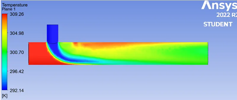
Plot 18. Contour temperature plot in long tee momentum ratio 4

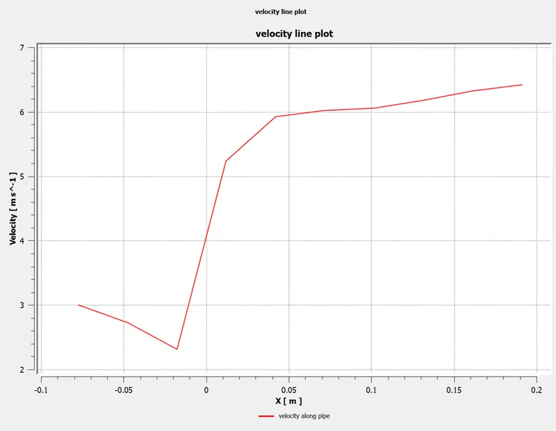
Plot 19. Velocity line plot long tee momentum ratio 4

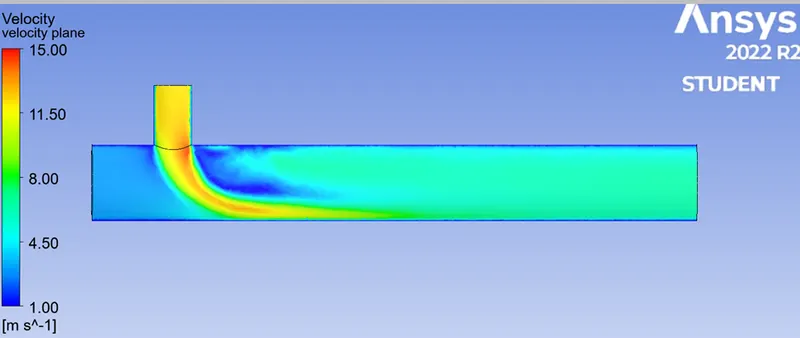
Plot 20. Velocity contour plot long tee momentum ratio 4

Convergence :

We carried out the visibility check on scaled residuals plot and that is our method for selecting where actual convergence happen so the point or the number of iteration where the changing of line or residuals stopped , that’s the iteration where convergence happened below in table shows some values about different iteration takes to converge , average outlet temperature and cell counts.

Parameters	Case 1. Short-T Momentum ratio 2	Case 1 Short-T Momentum ratio 4	Case 2 Long-T Momentum ratio 2	Case 3 Long-T Momentum ratio 4
Cell counts	106587 cells	106587 cells	289669 cells	289669 cells
Average outlet temperature	30.5553 C	27.6052 C	30.3968	30.6023
Number of iterations for convergence	150	1149	750	2000

Table. Case wise data table

Mesh independent study :

We carried out different meshing settings like changing of element sizes so we change it till 0.001 to 0.005 but it goes more and more finer and creates more elements which didn’t allow us to go through because student licence allows maximum element size till 51000, so when we goles below 0.0015 element size the elements exceeds size of 51000so we take 0.002 as element size and we get the values like nodes and number of element as we can see below in table

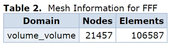
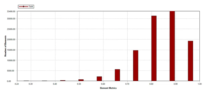
Chart of mesh elements

Effect of length and momentum ratio on results :

It is very basic and easy to say that yes it will effect on result if we change the length and momentum of pipe but we will see it number or values vies like how it behaves and what change occurs. so when hot air started to flow with velocity 3m/s with temperature of 36 C and mixed with cold air 19C with velocity of 3 with momentum 2 (velocity 6m/s) then there is sudden fall in temperature disturbance in velocity like some up-downs. So when it goes to end in short tee condition when it reaches till end the velocity goes to 6.1m/s. and just like that temperature started from hot end with 36 C and once it mixes with cold air of 19 C then the mix temperature falls to 20 C , and once it flows to end of pipe its mixed temperature gets 28 C now when we change its momentum and length the velocity started from 3m/s which goes till 6.3m/s in long tee with momentum ratio 4 and temperature falls gradually like starting from 36 C and falls till 26 C so we can clearly see the changes in numbers and results too.