Week 1- Mixing Tee

AIM:

To perform steady-state simulations to compare the mixing effectiveness of Tee joint of different lengths using Ansys Fluent.

DIFFERENT CASES TO SIMULATE:

1. Case-1

Short mixing tee with a hot inlet velocity of 3m/s.

Momentum ratio of 2, 4.

2. Case 2

Long mixing tee with a hot inlet velocity of 3m/s.

Momentum ratio of 2, 4.

SIMULATION PROCEDURE:

The CFD simulation is done using Ansys Fluent module available from the Workbench.

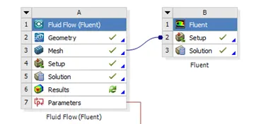
Fluid Model in Ansys Workbench

1. PRE-PROCESSING:

• BUILDING GEOMETRY: The given geometry of STEP format is imported to the SpaceClaim application available in the Ansys Workbench. The main objective of building geometries is to create the fluid domain. Using Volume extract feature from the Prepare tab, required fluid domain is created. Since Heat transfer parameters are not considered, fluid volume is alone sufficient for the Simulation. So the external wall is suppressed and Fluid volume is taken to the meshing.

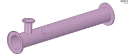
Above figures shows the TEE geometry and Fluid volume

• MESHING

The required fluid domain is meshed using standard options available in the Mesh tool. Mesh size of 3mm is used. It is to be ensured that mesh element quality should be at least 5%.

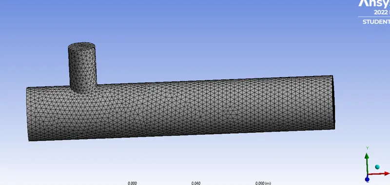
Meshed Fluid Volume

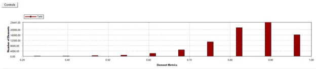
Element Quality Metrics

In our case, minimum mesh quality is higher than 29%. So our mesh is good to be considered for the Simulation. Next, to provide boundary conditions, named expressions are to be created on the required faces of the fluid volume as shown in the below image.

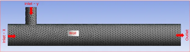
Named Expression on the Fluid Volume

2. SOLVING

Simulation is carried out in the setup option available in the Fluent Module.

1. In the first step, the setup type needs to defined. Here Pressure based stead state simulation is considered.
2. Since we are interested in capturing the temperature effects, we need to turn on the Energy equation. Also mixing happens in our volume, so Turbulence Model Should be enabled. As given in the problem statement, K-Epsilon Standard and K-Omega SST models are to be taken into Consideration. In the 1^st case, K-Epsilon is Considered.
3. For the simulation purpose, as mentioned before only fluid domain is considered. So in the cell zone condition Volume is predefined as fluid(Air).
4. Next, Boundary Conditions needs to be defined. In our problem statement, we are given with the hot inlet Velocity, Momentum ration and temperature values at both the Inlets. Based on the Momentum ratio value, Cold inlet velocity can be found. So the named expressions defined would be appearing in boundary conditions tab.

When Momentum ratio = 2

At Inlet-X

Hot inlet velocity = 3 m/s

Hot inlet temperature = 36 degC

At Inlet-Y

Cold inlet velocity = 6 m/s

Cold inlet temperature = 19 degC

At Outlet

Outlet Pressure = 0 Bar. G (open to Atmosphere)

Wall is considered as Stationary Wall

When Momentum ratio is considered as 4, only the Inlet-Y boundary conditions are modified.

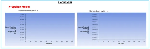
5. Default solution methods are followed for this simulation. In the report definitions, two surface reports are added. (i) Area weighted average of outlet temperature (ii) Standard deviation of outlet temperature.
6. Initialization: At t=0, initial variables are to be declared in the Mesh points. So hybrid initialization method is used. The main difference between hybrid and standard initialization is that Standard Initialization just fills the mesh points with a constant value for 1 iteration whereas hybrid initialization uses Euler method for 10 no. of iterations. When the no of inlet is more than 1, hybrid initialization is more preferred.
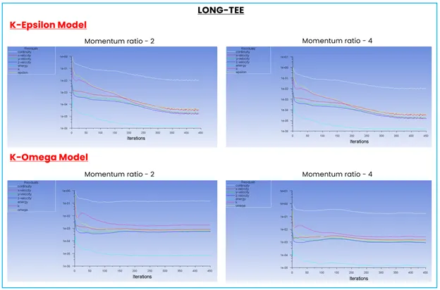
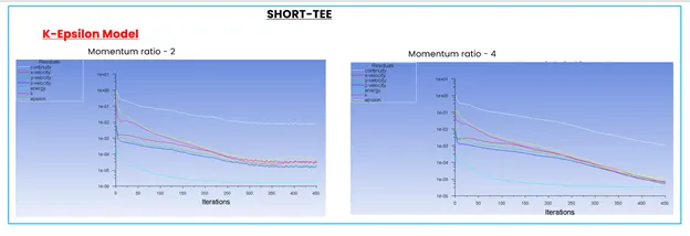
7. Once initialization is done, Simulation can be performed. Here to check the Convergence, initially we have considered 450 no of iterations. Based on the convergence, no of iterations can be altered after.

Similar procedure can be followed for different Momentum ratios.

3. Post-Processing

Once the solution is converged, required results can be transformed into a readable manner using post processing techniques. Ansys fluent has an Extensive option to do post-processing where different line or plane can be created inside the model to read the results.

In our case, Velocity and temperature contour plots on the cut planes along and across the pipe,

Velocity and temperature line plots along and across the length of the pipe are to be found.

RESULTS:

A. Comparison between K-Epsilon and K-Omega Model for Long-Tee Geometry

1. Convergence Plots

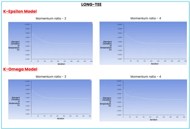
2. Standard deviation of Outlet temperature

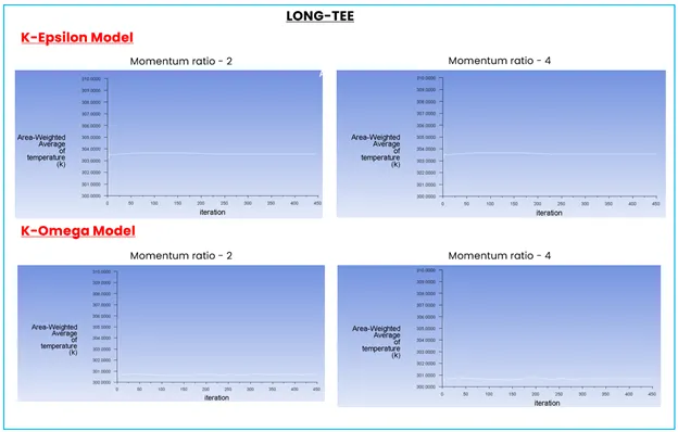
3. Area weighted average of Outlet temperature

K-Epsilon Model:

The K-epsilon turbulence model is the most common model used in CFD to simulate turbulent flow conditions. It is a two-equation model that gives a description of turbulence by means of two transport equations (PDEs).

(K) - turbulent kinetic energy), (Epsilon)- Rate of dissipation of turbulent kinetic energy.

k-omega SST

Shear Stress Transport (SST) is a variant of the standard k–omega model. Combines the original Wilcox k-w model for use near walls and the standard k– Epsilon model away from walls using a blending function, and the eddy viscosity formulation is modified to account for the transport effects of the principle turbulent shear stress. SST is recommended for high accuracy boundary layer simulations.

Reason to use K-Epsilon Model:

k-omega model of turbulence is capable of solving turbulence parameters very close to boundary or wall region. If we are interested to capture the phenomenon in such region, we have to have very fine mesh near to the wall, so that Y+ value should be as small as possible. on the other hand, k- epsilon provides standard results. Since our interest is to study the mixing phenomena along the length, we are proceeding with Standard K-Epsilon model.

B. Short TEE Results

1. Convergence Plots

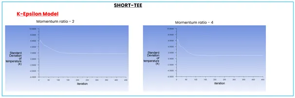
2. Standard deviation of Outlet temperature

3. Area weighted average of Outlet temperature

C. Contour graphs:

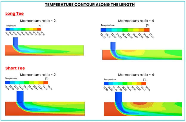
1. Temperature Contour along the length of TEE

2. Velocity Contour along the length of TEE

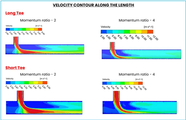
D. Velocity graph along the Length of TEE

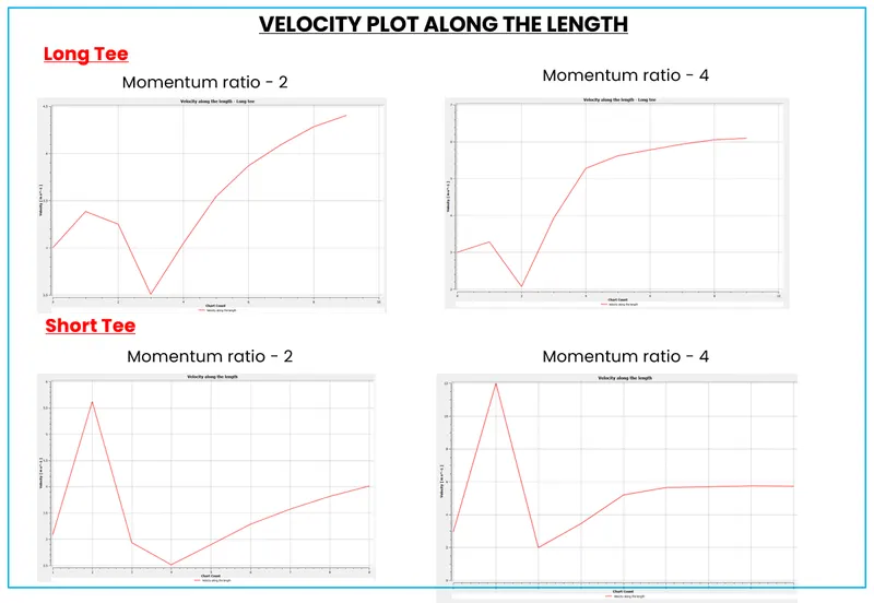
E. Temperature graph along the Length of TEE

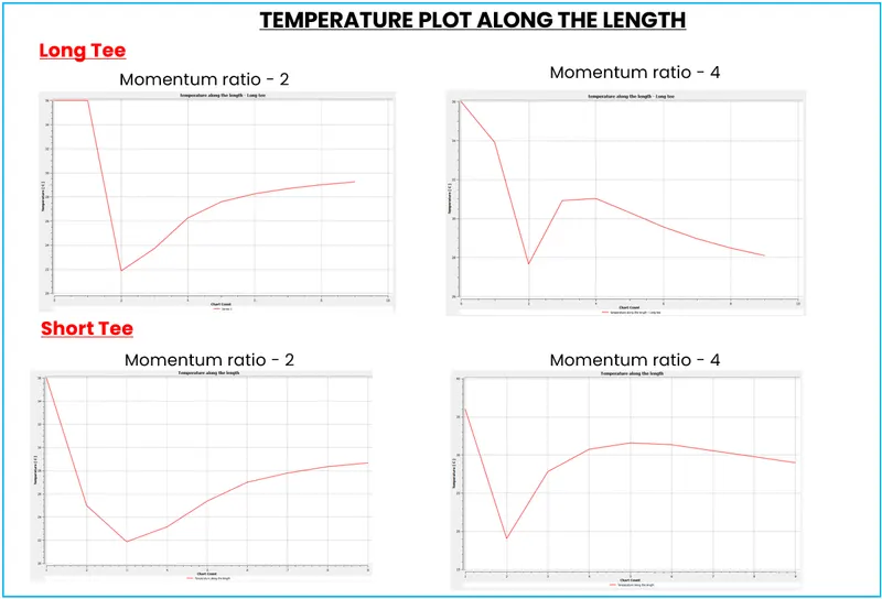
DISCUSSIONS:

1. Effect of length in Mixing:

This effect can be inferred based on the standard deviation value of the outlet temperature. In all the cases, the standard deviation of outlet temperature is stable after 125 no of iterations. The main criteria for better mixing is to have lower standard deviation value.

From the above results, it can be inferred that for momentum ratio = 2, the standard deviation value of outlet temperature is around 2 Kelvin whereas when Momentum ratio= 4, the standard deviation value is around 1 Kelvin after 125 no. of iteration. It can be concluded that length of the TEE is not much significant on mixing. Higher velocity flow shows better results in mixing. From the temperature contours also, we can infer the same.

2. Mesh independence study:

The Initial simulations were carried out for the mesh size of 3mm. But Grid independence study is done for Short tee with mesh size having 2mm, 2.5mm, 3mm, 4 mm and 4.5mm. In all the case the element quality was greater than 15%.

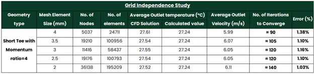
The above table shows the results for different mesh sizes. When element size is decreased, accurate results are obtained. For the given flow conditions, calculated value for the outlet temperature is 27.24°C. But for our standard mesh size = 3mm, the outlet temperature is 27.55 °C. So when the mesh size is decreased, obviously the better results are obtained. But computational time is higher. So one must be careful in choosing the type of element, mesh size for a particular problem to obtain better results