Week 1- Mixing Tee

Question: There are two versions of the mixing tee. One of them is longer than the other.

The aim is to set up steady-state simulations to compare the mixing effectiveness when hot inlet temperature is 360˚C & the Cold inlet is at 190˚C. Use the k-epsilon and k-omega SST model for the first case and based on your judgment use the more suitable model for further cases. Giving the reason for choosing a suitable model is compulsory.

• Case 1:

Short mixing tee with a hot inlet velocity of 3m/s.

Momentum ratio of 2, 4.

• Case 2

Long mixing tee with a hot inlet velocity of 3m/s.

Momentum ratio of 2, 4.

Momentum ratio = velocity at cold inlet / velocity at hot inlet

In a table, compare the following values from the 2 cases.

1. Cell count
2. Average outlet temperature
3. Number of iterations for convergence

Expected results:

1. Velocity and temperature contour plots on the cut planes along and across the pipe.
2. Velocity and temperature line plots along and across the length of the pipe.
3. Perform Mesh independent study for any one case.
4. Discuss the effect of length and momentum ratio on results.

Theory: The function of mixing tee is to allow proper mixing of hot and cold fluids to get the desired fluid at the outlet. By controlling the velocity of hot or cold air the resulting outlet temperature can be regulated.

Steps:

1. In Ansys Workbench, drag and drop Fluid Flow (Fluent) into Project Schematic.
2. Import the given CAD Model (Short Tee or Long Tee) into Spaceclaim for clean-up.
3. In Spaceclaim, extract fluid volume from the geometry by selecting the inlet/outlet edges together. After extraction, ensure to supress the solids in the CAD model for Physics so that they are not involved in the steps further. Then exit Spaceclaim.
4. Open Mesh generation module. Create Named Selections for Inlet X, Inlet Y, Outlet X and Wall.
5. Assign appropriate element size (2mm in this report) as per grid-dependency test and generate mesh. Ensure that the element metrics/quality is not lower than 5%. Exit Mesh module.
6. Set the following data in Fluent Module for the simulation of Short Mixing Tee.

Criterion	K-Epsilon	K-Omega
Solver Type	Pressure Based
Velocity Formulation	Absolute
Time	Steady
Viscous Model	K-Epsilon	K-Omega
Material	Air
Boundaries	Inlet X (Velocity Inlet) Velocity: 3m/s Temperature: 36˚C
	Inlet Y (Velocity Inlet) Velocity: 6m/s Temperature: 19˚C
	Outlet X (Pressure Outlet) Gauge Pressure: 0 Pa Walls: Stationary

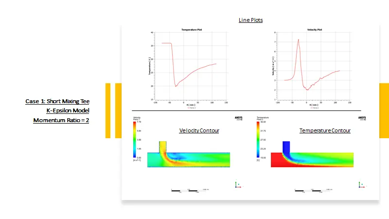
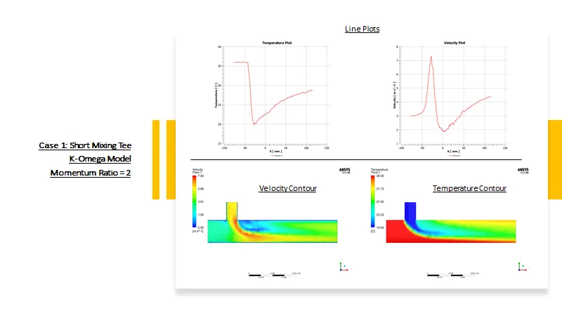
7. The above data is for the K-Epsilon vs. K-omega Viscous model comparison for Short Tee with Momentum Ratio = 2 [i.e., velocity at cold inlet (Inlet Y) ÷ velocity at hot inlet (Inlet X) = 2].
8. Solve the model after initializing by Hybrid Initialization.
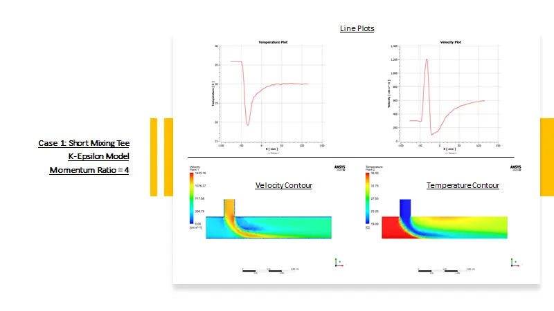
9. Repeat the above steps but with viscous method = K-Epsilon for Short Tee with Momentum Ratio = 4 i.e., velocity at inlet Y = 12m/s
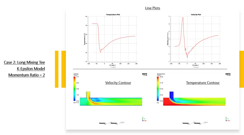
10. Repeat steps 1-8 but with viscous method = K-Epsilon for Long Tee with Momentum Ratio = 2 i.e., velocity at inlet Y = 6m/s
11. Repeat steps 1-8 but with viscous method = K-Epsilon for Long Tee with Momentum Ratio = 4 i.e., velocity at inlet Y = 12m/s

Results:

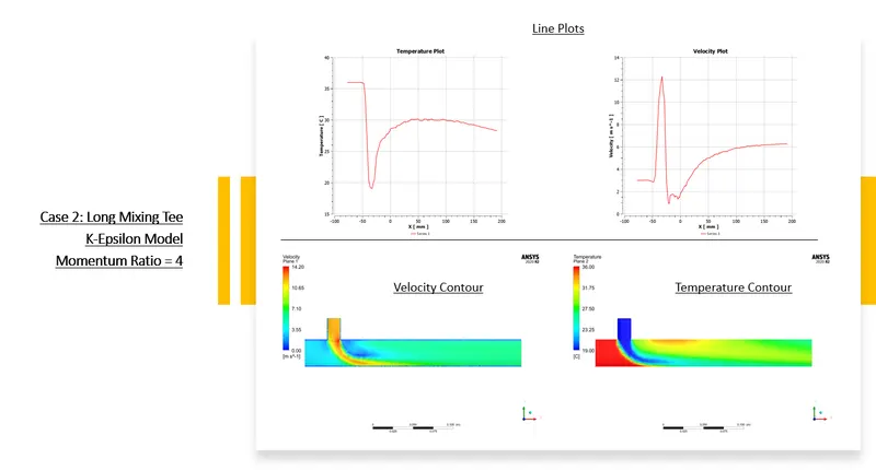
Conclusion:

Short Mixing Tee - Momentum Ratio = 2
Criterion	K-Epsilon	K-Omega
Cell Count	105858	105858
Average Outlet Temperature	303.5K	300.5K
Standard Deviation	1.7	3.5
Number of Iterations for Convergence	120	200

From the table above, we can see that the standard deviation of k-epsilon is lower than k-omega, hence k-epsilon has better mixing efficiency. The K-epsilon model also converges to the solution faster than k-omega model.

Therefore, K-epsilon model is more accurate and faster, and can be recommended for applications.

Model	Momentum Ratio	Cell Count	Average Outlet Temperature	Standard Deviation	No. Of Iterations for convergence
Short Mixing Tee	2	105858	303.5K	1.7	120
	4	105858	300.75K	1.45	100
Long Mixing Tee	2	105858	303.5K	1.25	125
	4	105858	300.75K	0.85	100

It can be seen that the mixing efficiency increases when the velocity of the cold fluid inlet increases. Hence higher the Momentum Ratio, better the mixing.

Temperature at outlet decreases with increase in Momentum Ratio.

The grid dependency test helps to conclude that a smaller overall element size will lead to greater accuracy of the result. As the element size decreases the error value (which is dependant on size of the cell) also decreases. Hence a finer grid size will result in accurate values. But with greater accuracy the computational time also increases. In this case we have chosen an element size of 2mm to strike a balance between computational time and result accuracy.