Week 1: Channel flow simulation using CONVERGE CFD
OBJECTIVE: To simulate airflow through a rectangular channel using CONVERGE CFD software for three different mesh resolutions (dx = dy = dz = 2e-4 m, 1.5e-4 m, and 1.2e-4 m). The goal is to analyze the development of flow characteristics-such as velocity, pressure, and mass flow rate-through detailed plots and animations.
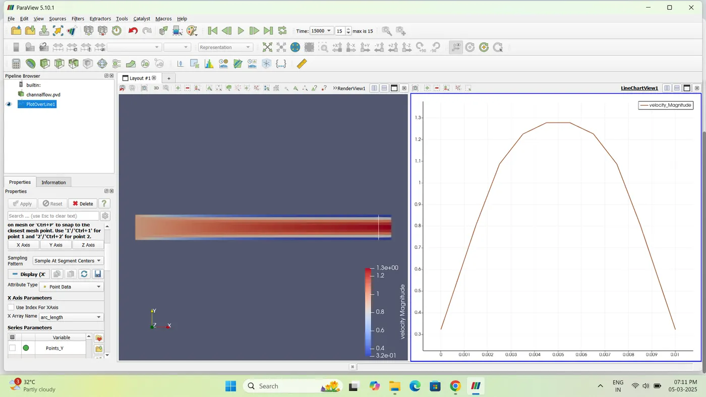
DESCRIPTION: The airflow inside a rectangular channel exhibits a parabolic velocity distribution due to the no-slip condition at the walls. The velocity is zero near the walls and increases towards the center of the channel. This simulation assumes two-dimensional flow, with variation only in the X and Y directions. No variation is considered along the Z-direction.
CASE SETUP:
1. Geometry Creation: -
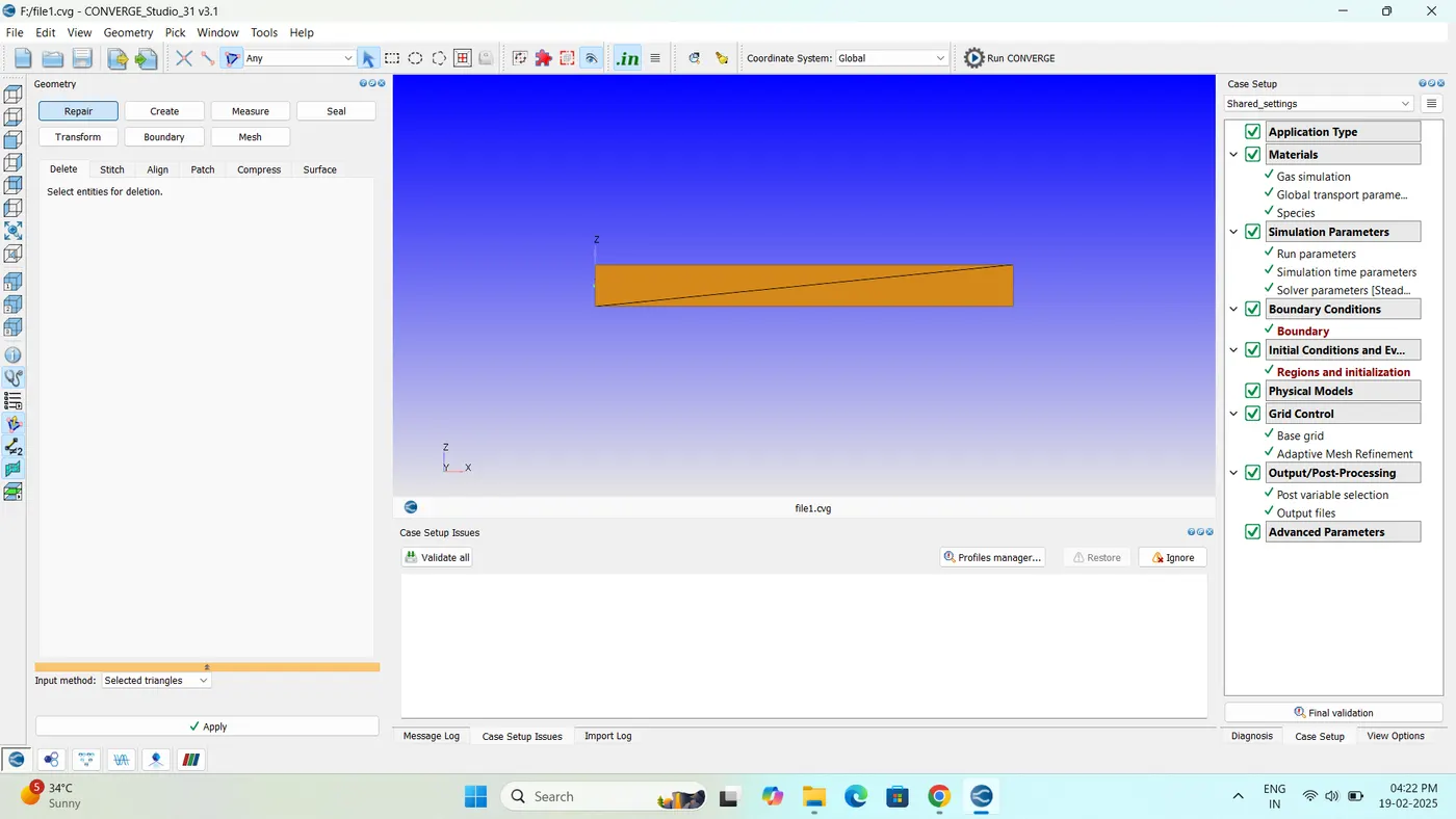
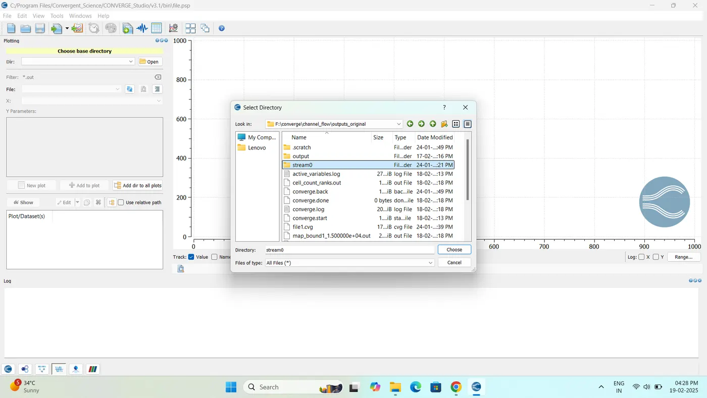
A rectangular box is created using the Create
> Box tool. - The surfaces are refined and combined to define boundaries.
2. Boundary Creation:
- Boundaries are created and flagged accordingly
: - ID 1: Inlet - ID 2: Outlet - ID 3: Top and Bottom walls - ID 4: Front and Back (2D boundaries)
- Normals are oriented to ensure flow direction is correctly represented.
- Geometry is validated using diagnostics.
3. Simulation Setup:
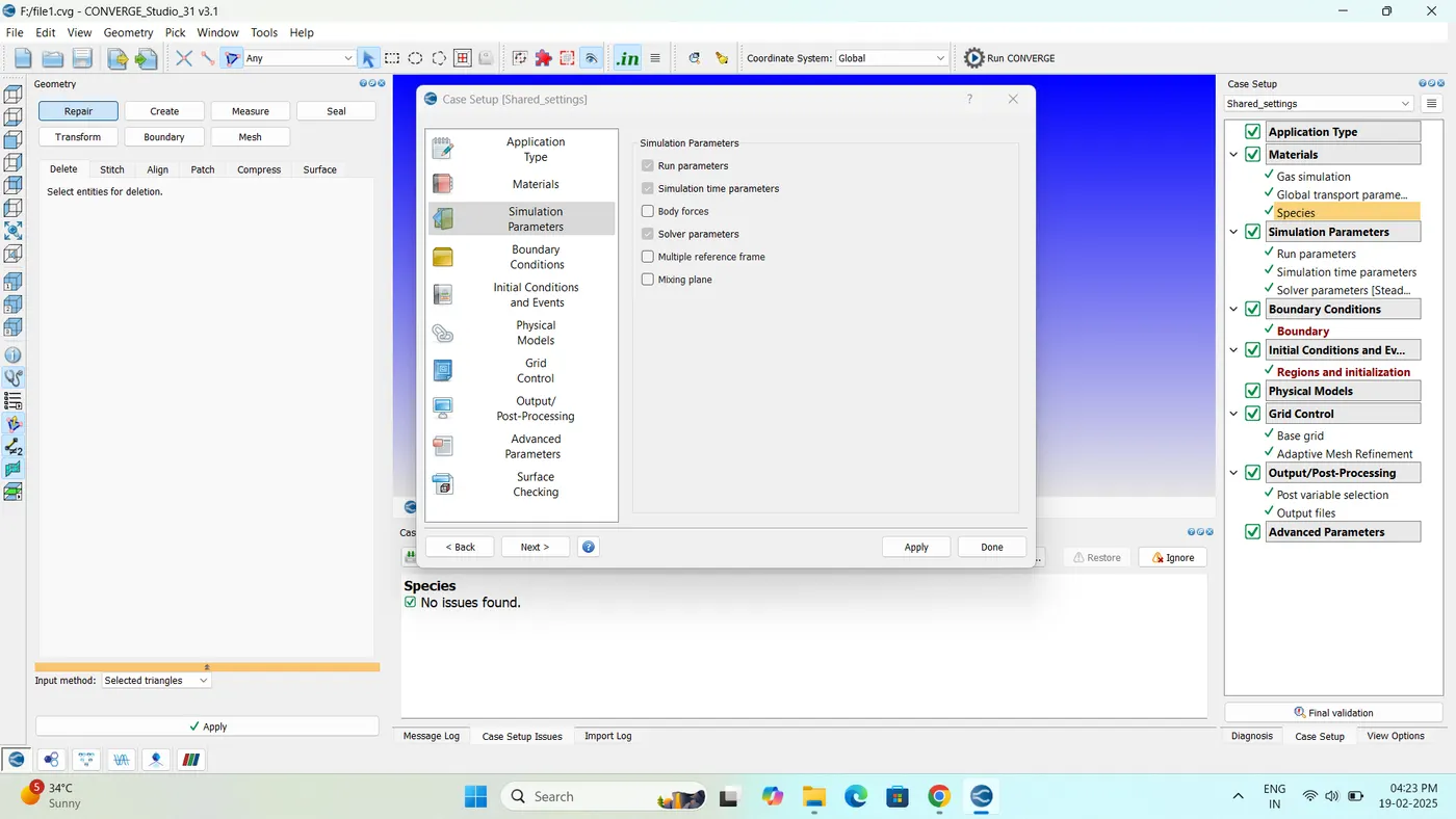
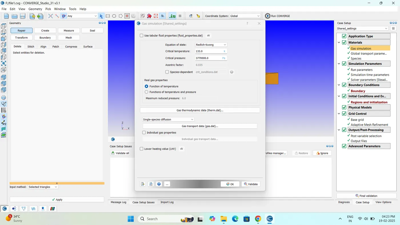
- Material: Air (no reaction mechanism)
- Flow Physics: Steady-state, compressible, full hydrodynamic
- Turbulence model: Disabled (laminar flow assumed)
4. Boundary Conditions: -
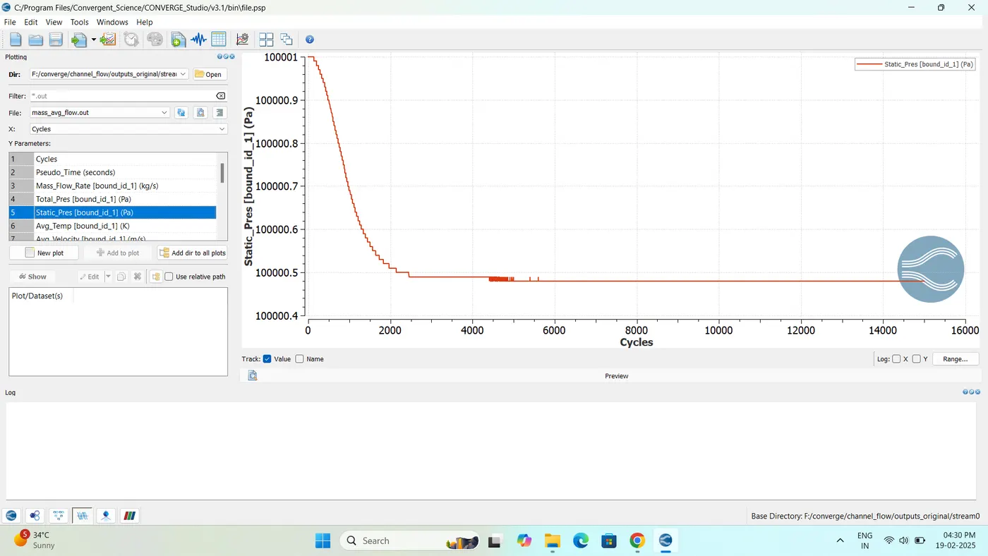
Inlet: Inflow boundary, pressure set to 100001 Pa
- Outlet: Outflow boundary, pressure set to 100000 Pa
- Top & Bottom: Wall boundary
- Front & Back: 2D boundary
5. Initialization and Grid Setup:
- Species mass fractions of O2 and N2 are initialized.
- Base grid: X-direction - 100 cells (0.1/100 = 0.001 m), Y-direction - 10 cells (0.01/10 = 0.001 m)
6. Post-Processing: - Post variables include O2 and N2 mass fractions.
- 3D data output interval set to every 150 time steps.
7. Solver Execution:
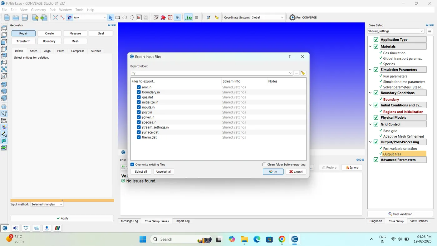
- Simulation run using mpiexec.exe and converge.exe
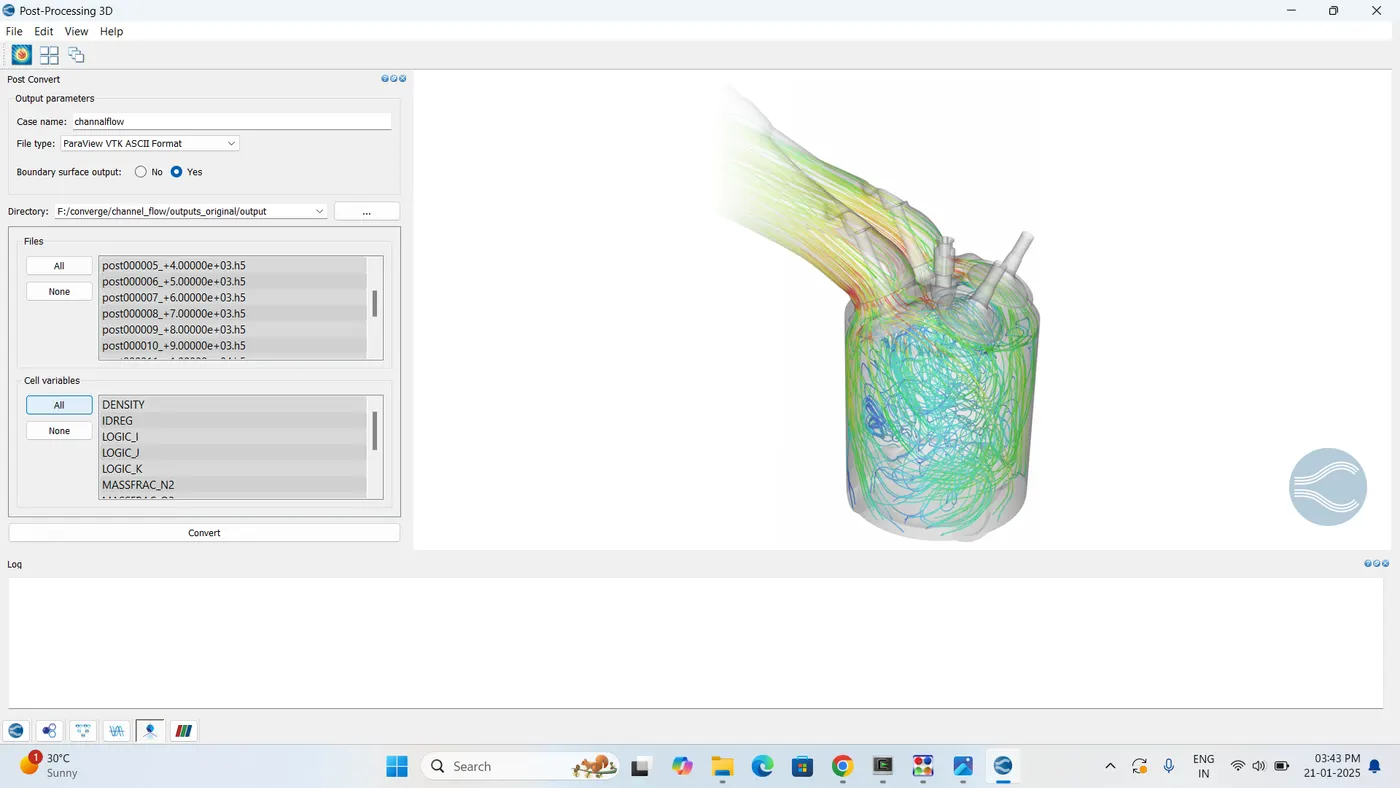
- Post-processing done using post_convert_30_serial_64.exe
SIMULATION CASES:
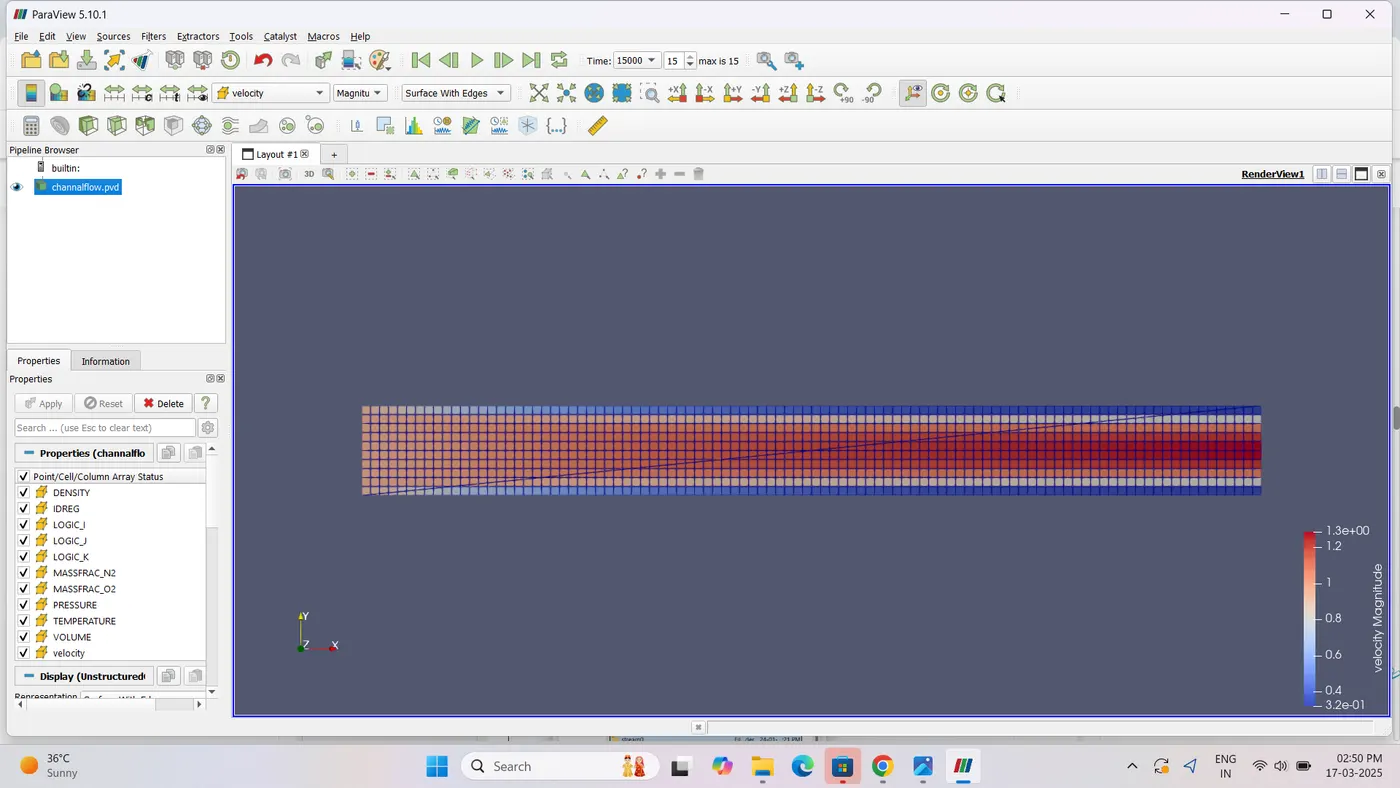
"Structured mesh generated for rectangular channel with grid size 2e-4 m."
Case 1: Mesh size = 2e-4 m
- Velocity Contour - Pressure Contour
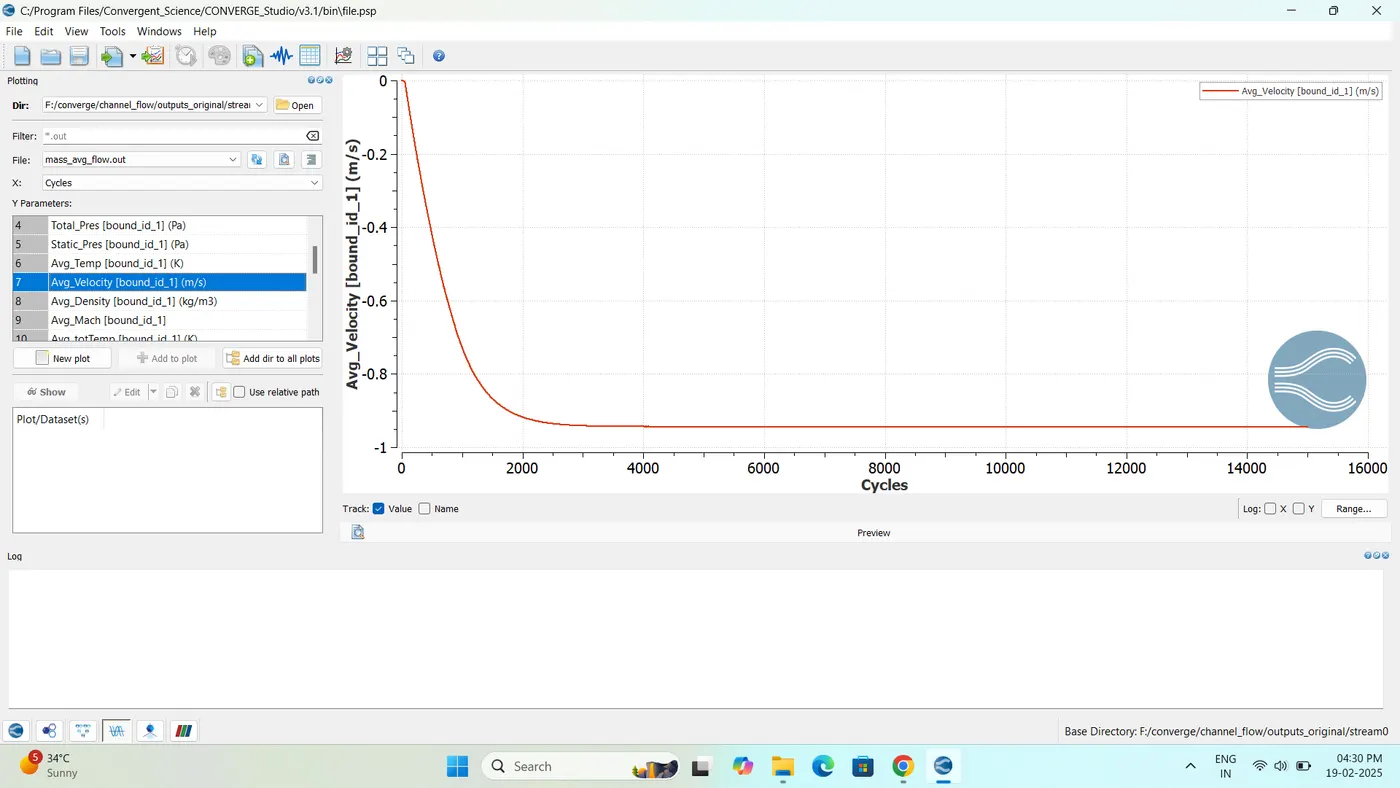
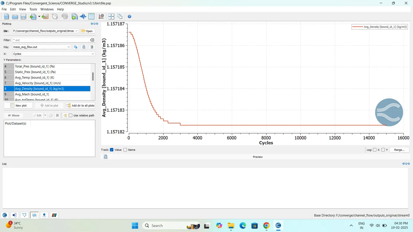
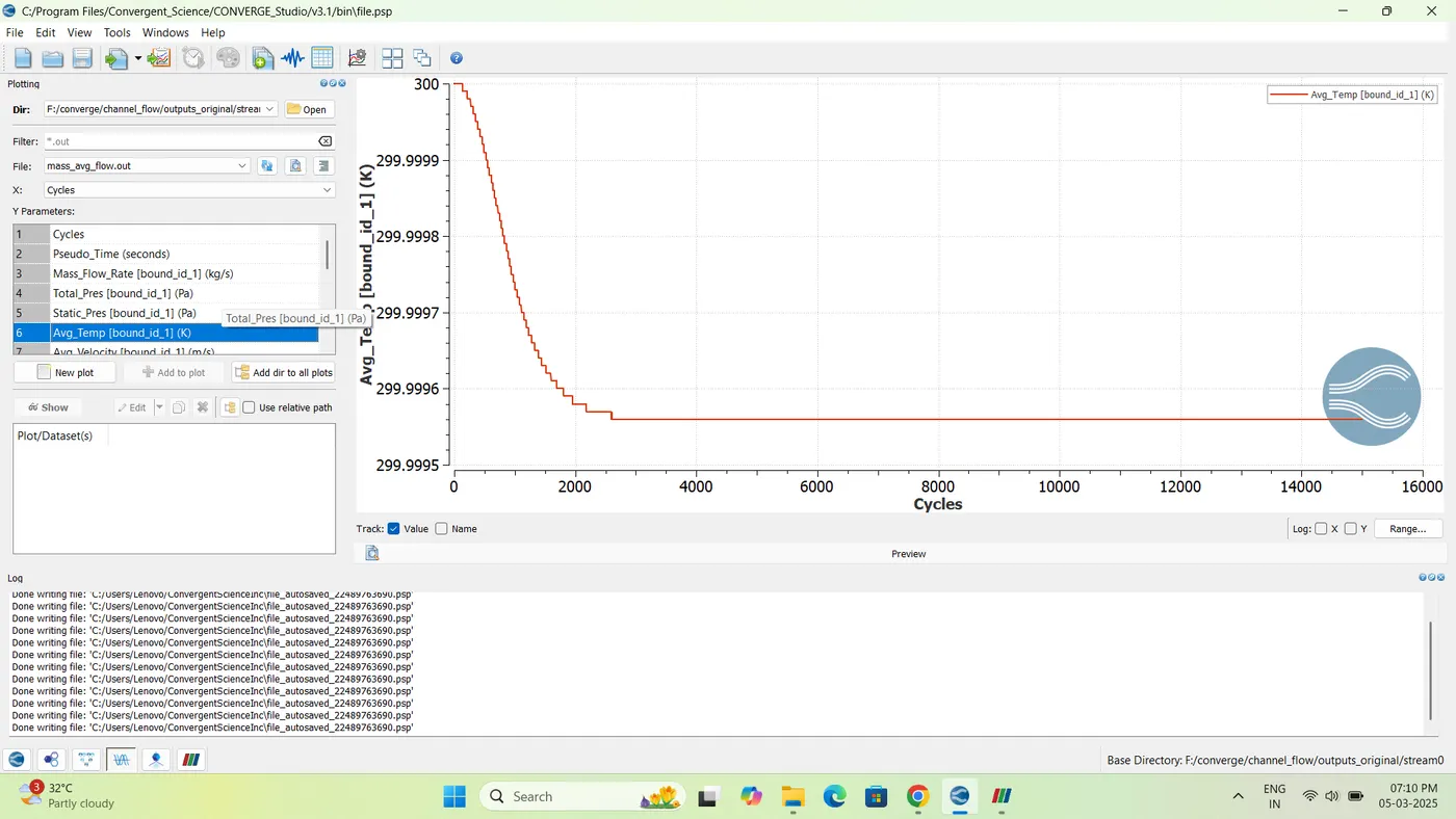
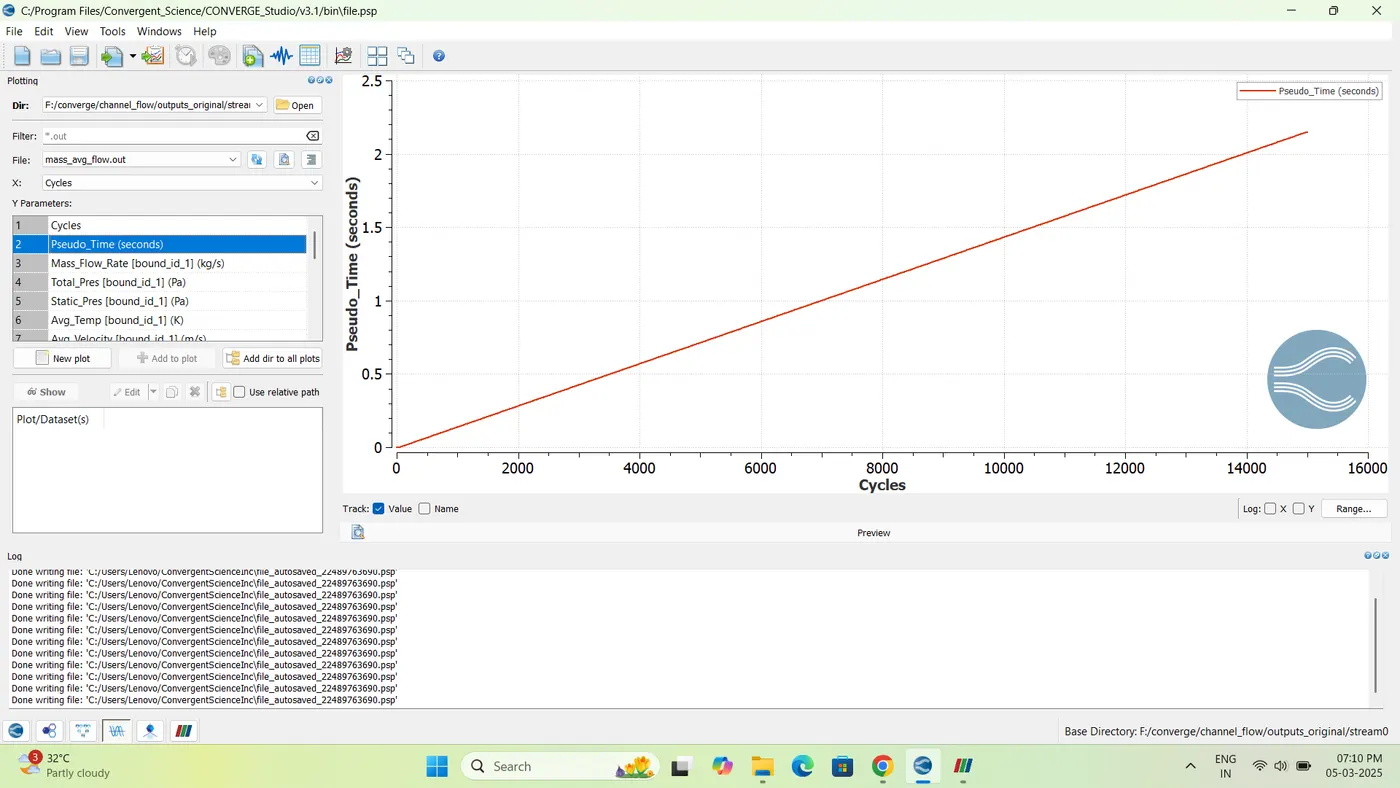
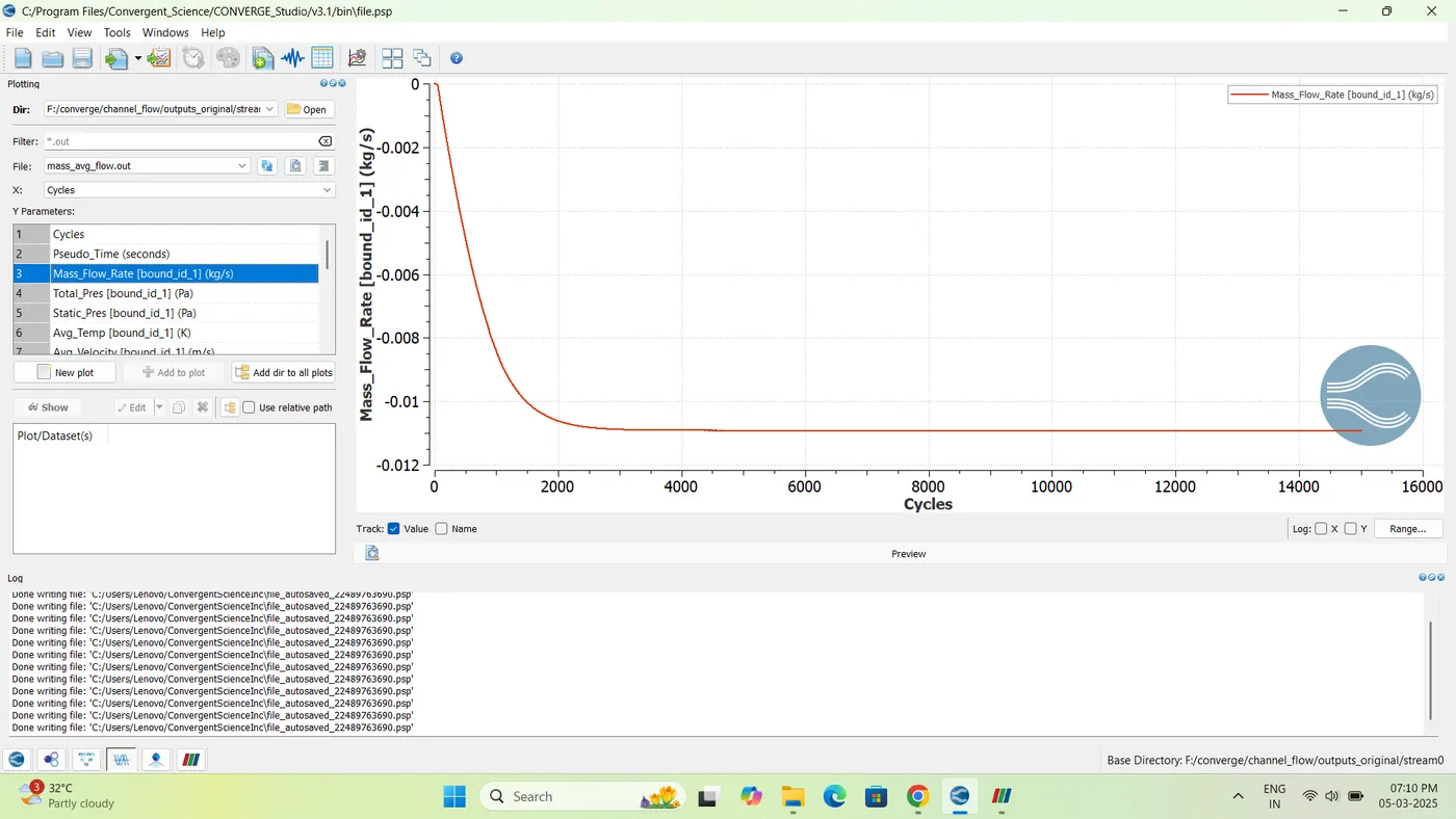
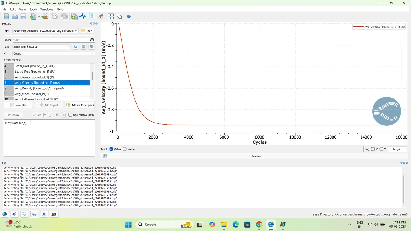
- Velocity plots at Inlet, 0.05 m, Outlet - Mass Flow Rate: Inlet & Outlet
- Average Velocity: Inlet & Outlet
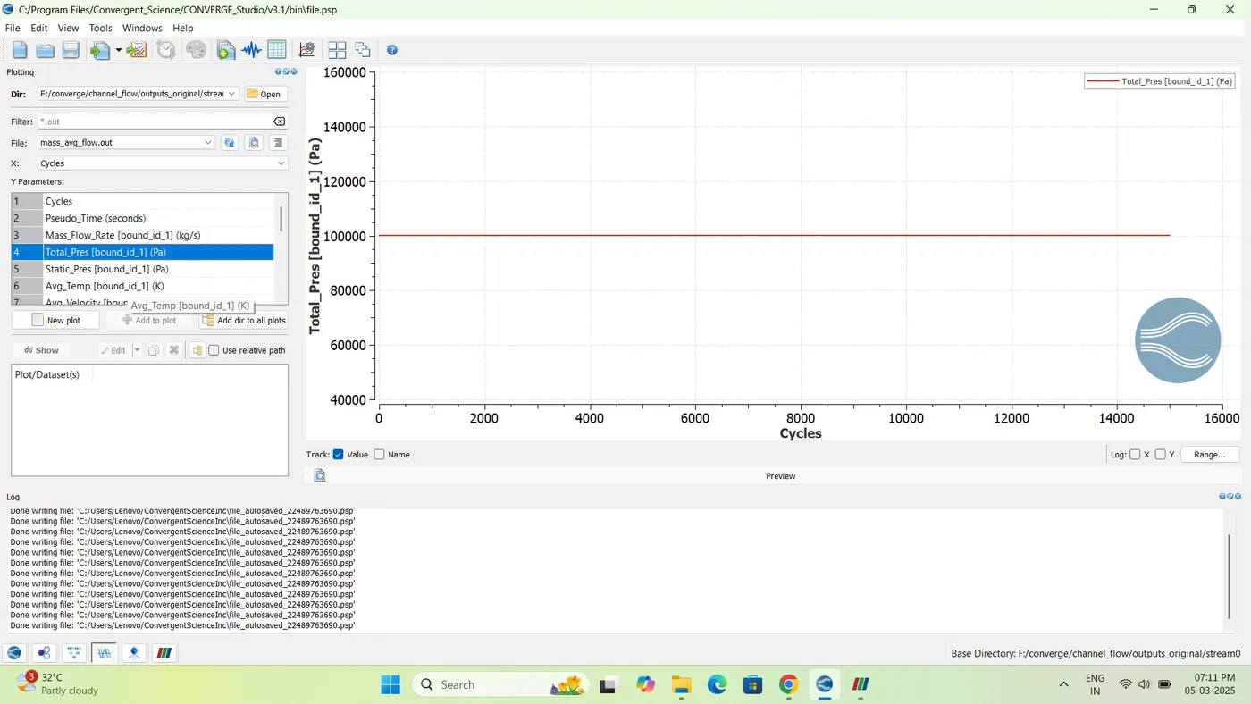
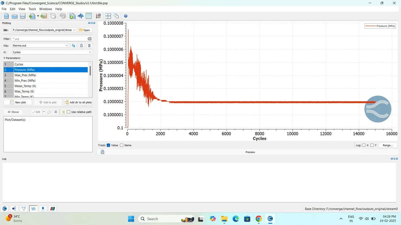
- Total Pressure: Inlet & Outlet
- Cell Count
Case 2: Mesh size = 1.5e-4 m
- Same parameters and plots as Case 1 Case
3: Mesh size = 1.2e-4 m
- Same parameters and plots as Case 1
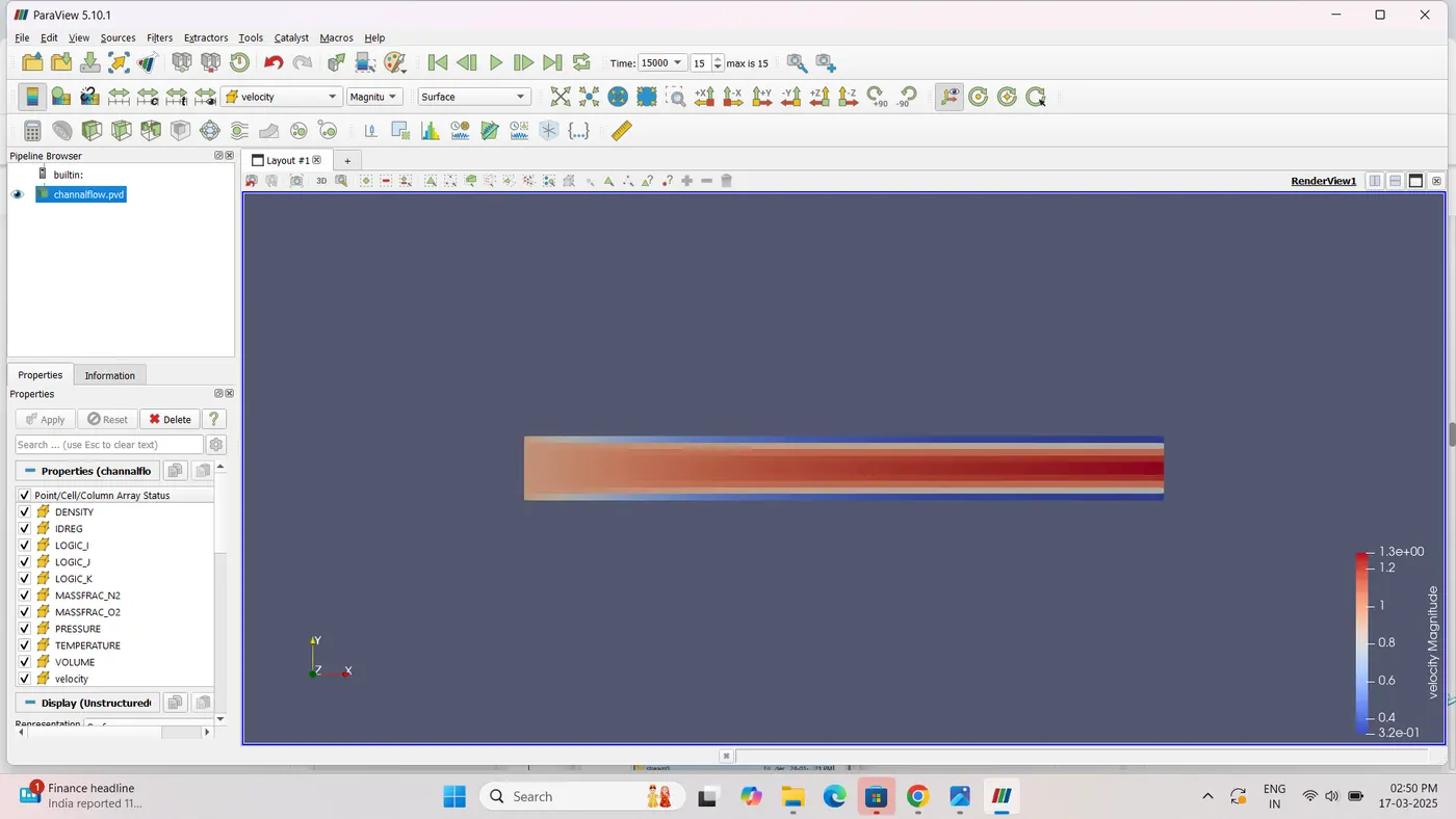
Velocity Contour (CASE-1 and 2,3)
Velocity Contour (CASE-2)
Velocity Contour (CASE-3)
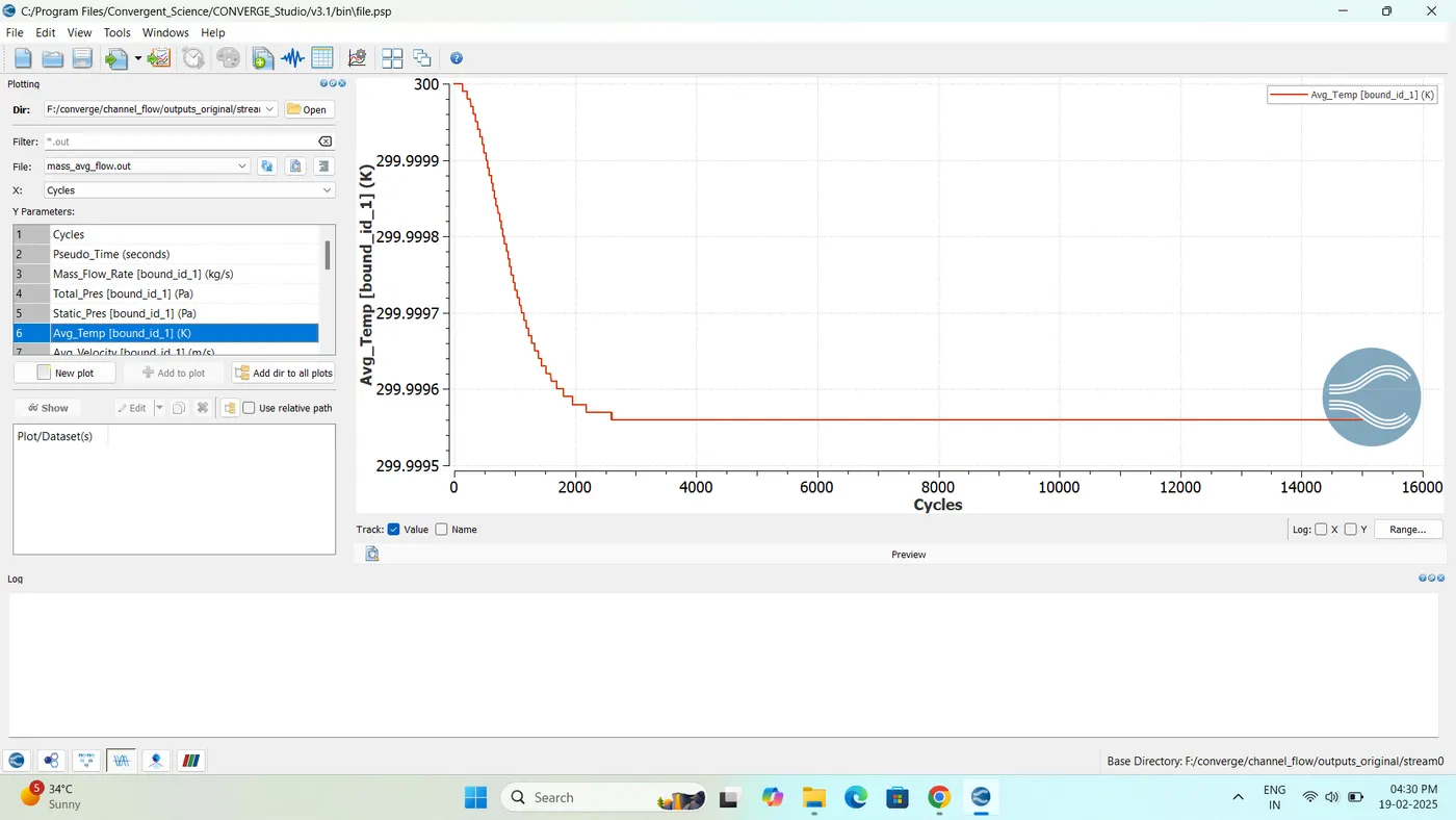
OBSERVATIONS AND CONCLUSION:
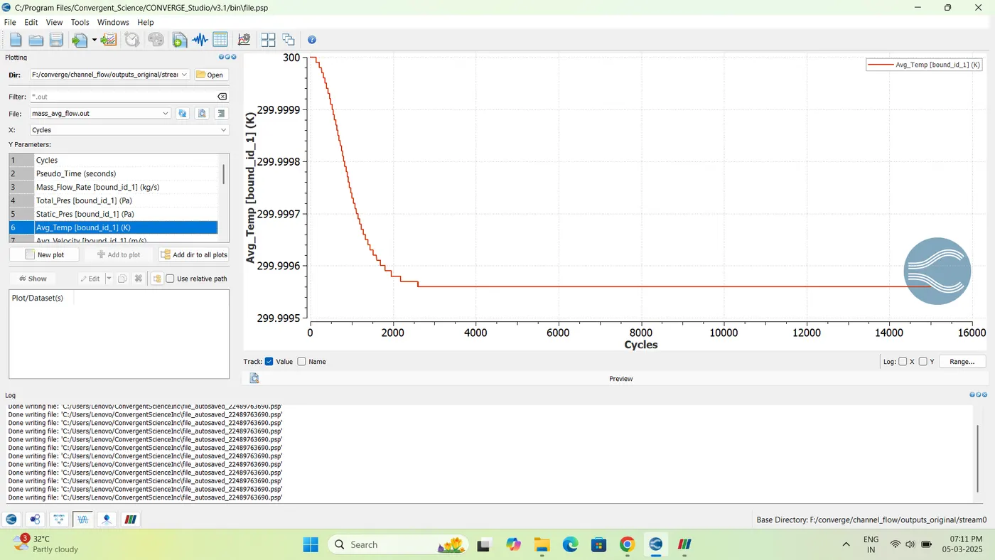
- The airflow is driven by pressure difference across the channel.
- Velocity contours confirm development of a parabolic profile due to no-slip condition at walls.
- Boundary layers form near the walls, with increasing thickness downstream.
- Mass flow rate and average velocity profiles at inlet and outlet validate conservation of mass.
- Total pressure remains constant at inlet, with slight variation at outlet.
- Constant cell count indicates mesh stability.
- Finer mesh improves accuracy but increases computational cost.
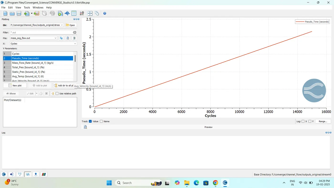
- Animations demonstrate the gradual formation of velocity profiles and flow characteristics over time.