Week 1: Channel flow simulation using CONVERGE CFD

Channel flow simulation

Objectives:

1. To set up Channel flow simulation using Converge Studio.

2. Run the case for following mesh sizes

• dx = 2e-4m, dy = 2e-4m, dz = 2e-4m
• dx = 1.5e-4m, dy = 1.5e-4m, dz = 1.5e-4m
• dx = 1.0e-4m, dy = 1.0e-4m, dz = 1.0e-4m

3. Postprocess the results with plots for velocity, pressure, mass flow rate, and total cell count.

Channel Flow:

Flow through a channel is one of the benchmarking simulations in the field of CFD to test and validate the numerical models. Here, the objective is to setup the same using a commercial tool, CONVERGE and extract the results for various mesh sizes.

Geometry:

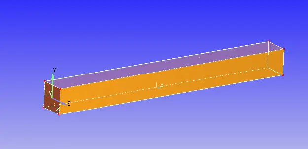
Fig. Geometry of Channel

• The above given geometry measures as follows: l_x=0.1m, l_y=0.01m, l_z=0.01m

Boundary Conditions:

Boundary	Conditions
Inlet	Pressure 100001 Pa
Outlet	Pressure 100000 Pa
Top and Bottom Faces	No slip wall
Right and Left Faces	2D Symmetry condition

From the boundary conditions, it is evident that the case is assumed with a symmetry boundary condition such that it is simplified numerically for faster computation with no compromise on results.

Material: The fluid across the domain is Air.

Simulation Setup:

• Steady State Simulation
• Density Based Solver is used as it is more robust in this particular tool. However, in general, pressure based solvers are used for low speed simulations whereas density based solvers are used for high speed flows such as flow through nozzles, aerodynamics of airfoils etc.
• Steady state is monitored based on the values mentioned in the below figure.

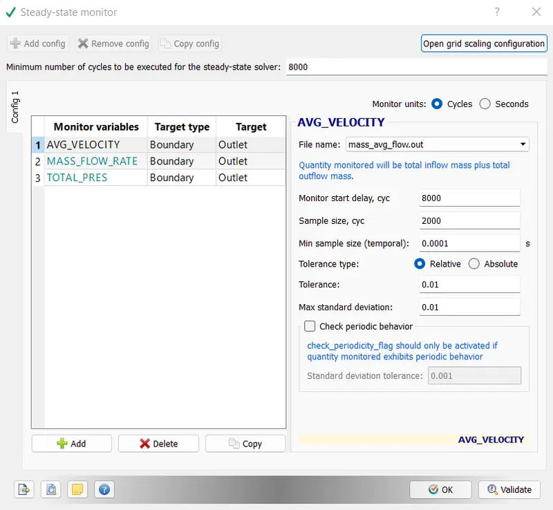
• Here, minimum number of cycles to be executed is set to 8000. The solution obtained at each iteration gets monitored only after this value of 8000 and compared whether it is below the tolerance limit. Sample Size is set to 2000 cycles meaning that only if the error below the tolerance is maintained for 2000 consecutive cycles, then only the computation is terminated.
• Tolerance limit and desired variables to be monitored are assigned as per computation power and desired accuracy.

Simulation time parameters:

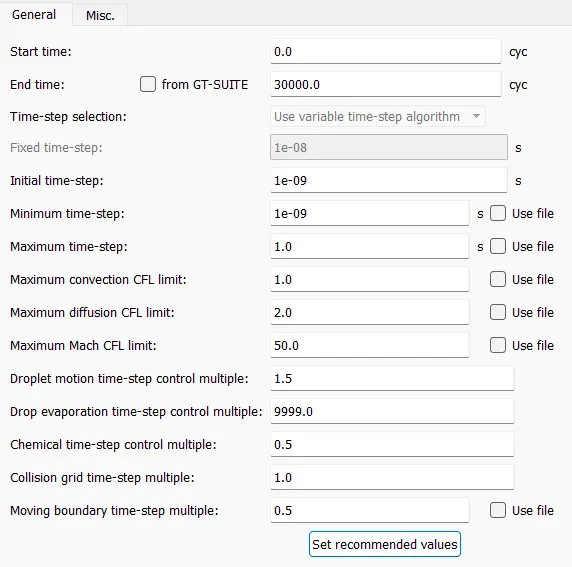
• Maximum number of cycles is set to 30000 but this may vary for different sizes of grids in order to achieve convergence.
• Minimum and Maximum time steps are 1e-09s and 1s respectively.
• Maximum convection CFL limit is set to 1 and Maximum diffusion CFL limit is set to 2. Other values are set to default.

Initial conditions:

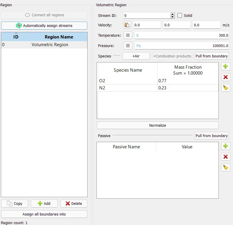
In order to initiate the numerical computation, initial conditions are defined. Here, region pressure is set equal to inlet pressure (100001 Pa), and all the boundaries are defined as a single volumetric region.

Case setups and results:

Case 1: dx=2e-4m dy=2e-4m dz=2e-4m

Above is the mesh structure of a uniform grid (across 3 directions) with cells of dimension 2e-4m.

Development of Velocity contour (Click here for detailed view)

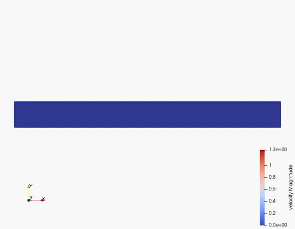
Velocity contour (fully developed):

At x= 0m At x= 0.025m At x= 0.05m At x= 0.075m At x= 0.1m

Inference (I):

From the above plots, the development of velocity is distinguished across the length of the channel. Initially, at x=0, velocity is almost constant. Upon further movement along the axial direction, it is evident that the velocity at the axial centre of the channel increases while the velocity near the walls is constant or zero due to the formation of boundary layers.

Development of Pressure contour (Click here for detailed view)

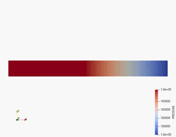
Pressure contour (fully developed):

Pressure variation across length:

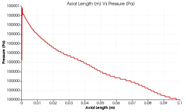
Inference (II): Pressure and velocity are inversely proportional. As the velocity at the outlet increases, pressure decreases. In this case, it is user-defined here and the plots are in correlation to the same.

Case 2: dx=1.5e-4m dy=1.5e-4m dz=1.5e-4m

Above is the mesh structure of a uniform grid (across 3 directions) with cells of dimension 1.5e-4m.

Development of Velocity contour (Click here for detailed view)

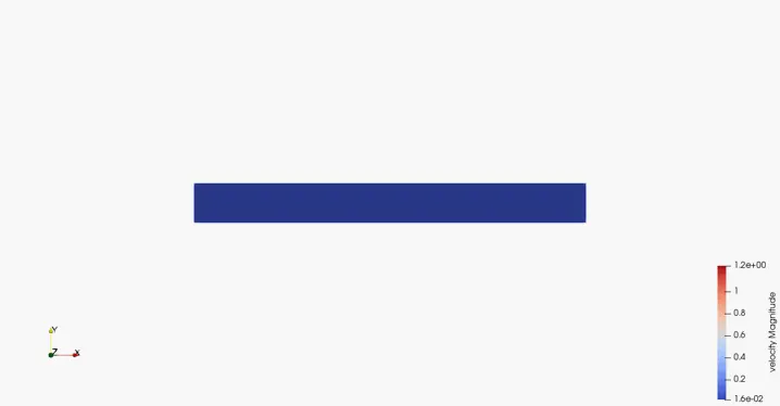
Velocity contour (fully developed):

At x= 0m At x= 0.025m At x= 0.05m At x= 0.075m At x= 0.1m

Inference (III):

Similar to inference (I), the velocity profile remains the same. However, the solution has shifted from 1.3 m/s to 1.2 m/s. The lower the grid size, the higher the accuracy. But in this case the change is due to a minor issue in the grid which is discussed below as a special case.

Development of Pressure contour (Click here for detailed view)

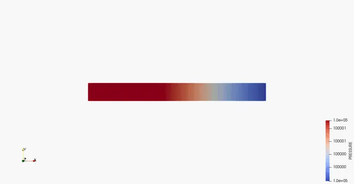
Pressure contour (fully developed):

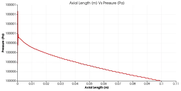
Inference (IV): Similar to inference (II), the pressure profile along axial length almost remains the same. But a clear difference can be observed in the colours. Pressure is higher only at the inlet (0m) but reduces quickly throughout the domain.

Case 3: dx=1e-4m dy=1e-4m dz=1e-4m

Above is the mesh structure of a uniform grid (across 3 directions) with cells of dimension 1e-4m.

Development of Velocity contour (Click here for detailed view)

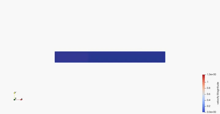
Velocity contour (fully developed):

At x= 0m At x= 0.025m At x= 0.05m At x= 0.075m At x= 0.1m

Inference (V): Velocity at the outlet is 1.059 m/s as against 1.054 m /s for case 1. Generally, the output of the finest grid is accurate but here the significance of the difference is much lesser.

Development of Pressure contour (Click here for detailed view)

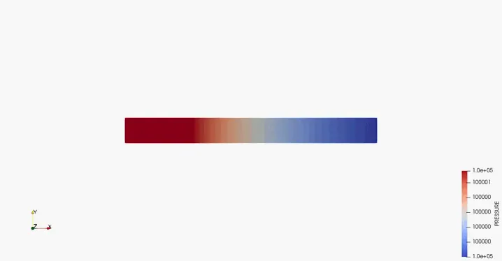
Pressure contour (fully developed):

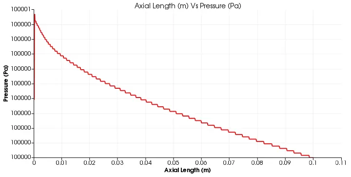
Inference (VI): The pressure fluctuations at the inlet seems to be lesser than in other cases due to the finer grid level. In terms of magnitude, there is not much of a significant difference from other cases.

Total Pressure:

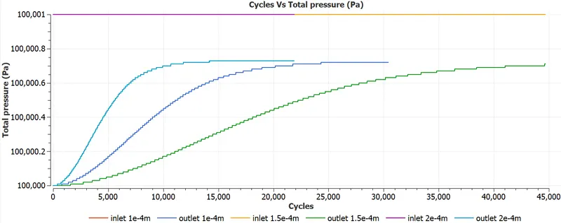
As per the boundary conditions, inlet is set higher than the outlet. The outlet pressure is converging between 100000.6 and 100000.8 Pa. Convergence of 2e-4m grid is much faster than the other two grids which is pretty much obvious. However, convergence of 1.5e-4m is taking longer than 1e-4m which is investigated as a special case at the end.

Average Velocity:

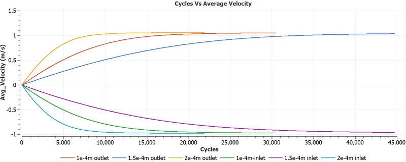
The convergence of velocity is between 0.8 to 1m/s at the outlet and -0.8 to -1 m/s at the inlet. Values of 1e-4m grid can be considered as the correct solution.

Mass Flow rate:

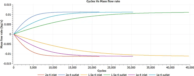
Mass flow is conserved in all 3 cases (i.e., mass flowing through inlet is equal to the mass flowing through outlet)

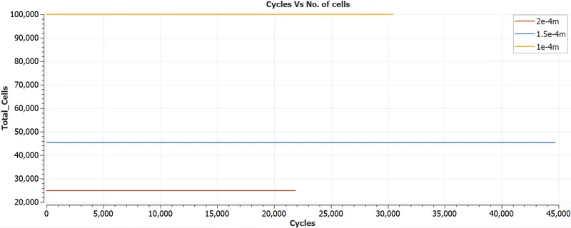
No. of cells:

Special Case:

In general, number of cycles taken for convergence increases as the grid size decreases. From the above plots we have a contradiction to the previous statement. Case 2 and 3 having mesh of size 1.5e-4m and 1e-4m respectively does not follow the general trend. This is due to the fact of aspect ratio.

Number of cells across a direction 'n' = (x/dx)+1, where x is the total length, dx is the grid size

for mesh size of 1.5e-4m, along the x direction, n = 667.666 cells. Cell counts cannot be in decimal. So converge adaptive mesh refinement technique tries its best to accommodate the number of cells in a given length. This increases the aspect ratio of few cells.

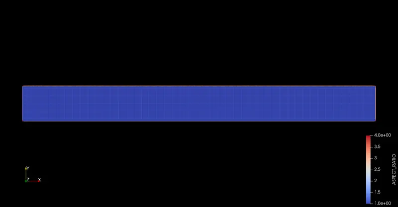
Aspect ratio is the ratio of Maximum edge length to the minimum edge length of an element. This has to be ~1 for smooth convergence of the solution. From the above figure, it is evident that it is almost 4 at the walls which are not desirable. So this affects the convergence of the case with a mesh 1.5e-4m leading to more iterations than case 3.

Results:

1. Velocity at the outlet increases while it gets reduced at the walls due to the formation of the boundary layer.

2. Pressure acts inversely with velocity. It decreases at the outlet whereas it almost stays constant at the inlet.

3. No. of cycles increases as the grid size decreases. However, cell count should be maintained as a whole number to avoid unnecessary conflicts.

4. Lower the grid size, higher the accuracy. Here, the results of 1e-4m grid should be accurate than the other two.