Using Genetic Algorithm in MATLAB to find the Global Maxima of stalagmite function and optimize it
Objective :
- to find the global maxima of the stalagmite function
- to optimize the stalagmite function
- to use the genetic algorithm in MATLAB
Stalagmite Function:
`f ( x , y ) = f 1 , x f 2 , x f 1 , y f 2 , y`
`f 1 . x = [ sin ( 5.1 π x + 0.5 ) ] ^6`
`f 1 . y = [ sin ( 5.1 π y + 0.5 ) ] ^6`
`f 2 . x = exp [ − 4 ln ( 2 ) ( x − 0.0667 ) ^2/ 0.64 ]`
`f 2 . y = exp [ − 4 ln ( 2 ) ( y − 0.0667 ) ^2/ 0.64 ]`
The given stalagmite function, of which we need to find the Global Maxima by using the Genetic Algorithm.
Creating the function named stalagmite:
function [f] = stalgamite_function(input_vector)

x = input_vector(1);
y = input_vector(2);

f1x = (sin(5.1*pi*x + 0.5))^6;
f1y = (sin(5.1*pi*y + 0.5))^6;
f2x = exp(-4*log(2)*(x - 0.0667)^2/0.64);
f2y = exp(-4*log(2)*(x - 0.0667)^2/0.64);

f = -(f1x*f1y*f2x*f2y);
end
Plotting the function by passing input arguments to the functions:
clear all
close all
clc

x = linspace(0,0.6,150);                                %Assigning input vectors
y = linspace(0,0.8,150);
num_iteration = 50                                      %number of the iterations to be done

[xx yy] = meshgrid(x,y);                                %Creating 2D vector array from single
for  i = 1:length(xx)                                   %loop to calculate function values for all input arguments
    for j = 1:length(yy)                                %we have nested the loop, to calculate all the possible combinations
        input_vector(1) = xx(i,j);
        input_vector(2) = yy(i,j);
        f(i,j) = stalgamite_function(input_vector);
    end
end
figure(1)
surfc(x,y,-f)                                          %Surface plot
colorbar
xlabel('x-values')
ylabel('y-values')
zlabel('function-values')
title('stalagmite function')
shading interp                                        %to remove the countour lines from the plot

[x_output , fval] = ga(@stalgamite_function,2)        %GA to claculate the maximum fitness value
%Above values is highly fluctuating 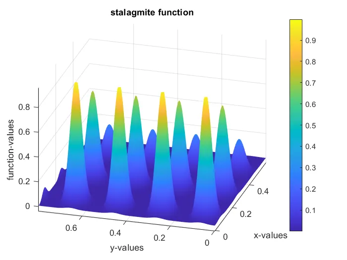
fig. Surface plot of the Stalagmite function
for that purpose, we are using genetic algorithm in MATLAB, Global Optimization Toolbox
Genetic Algorithm :
The genetic algorithm is a method for solving both constrained and unconstrained optimization problems that is based on natural selection, the process that drives biological evolution. The genetic algorithm repeatedly modifies a population of individual solutions. At each step, the genetic algorithm selects individuals at random from the current population to be parents and uses them to produce the children for the next generation. Over successive generations, the population "evolves" toward an optimal solution.
The genetic algorithm uses three main types of rules at each step to create the next generation from the current population:
-
Selection rules select the individuals, called parents, that contribute to the population at the next generation.
-
Crossover rules combine two parents to form children for the next generation.
-
Mutation rules apply random changes to individual parents to form children.
Terminologies :
Here, The stalagmite function is termed as the Fitness Function, as it is the function we want to optimize.and we are applying this function for certain vector(x(i),y(j)) it is specified below in the code, it termed as Individuals . The combined all individuals is termed as Population. The fitness value of an individual is the value of the fitness function for that individual. Here, we are finding out that maximum of the fitness of the function, so the fitness value of the population is the largest fitness value of the fitness in the population.
Working of the Genetic Algorithm :
The following outline summarizes how the genetic algorithm works:
-
The genetic algorithm starts by taking some random initial population.
-
The algorithm then creates a sequence of new populations. At each step, the algorithm uses the individuals in the current generation to create the next population. To create a new population, the algorithm performs the following steps:
-
Scores each member of the current population by computing its fitness value. These values are called raw fitness scores.
-
Scales the raw fitness scores to convert them into a more usable range of values. These scaled values are called expectation values.
-
Selects members, called parents, based on their expectations.
-
Some of the individuals in the current population that have lower fitness are chosen as elite. These elite individuals are passed to the next population.
-
It produces children from their parents. Children are produced either by making random changes to a single parent—mutation—or by combining the vector entries of a pair of parents—crossover.
-
Replaces the current population with the children to form the next generation.
-
-
The algorithm stops when one of the stopping criteria is met.
The Genetic Optimization Algorithm is used to calculate the minimum of the function, In this task we have to calculate the Global maximum.
1)Optimization_1 :
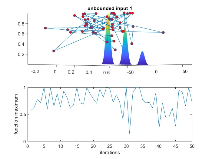
In this, we have run the code for the 50 iterations, unbounded, and as we know the GA taken a random input population and tried to calculate the best fitness value. and plotted it on the same surface plot and also with that we have plotted the graph of the value of function maximum with respect to the number of iteration.
Code for Optimization_1:
%% Optimization_1
tic                                                     %timer_start
%to caluculate the maximum fitness value but by using loop (50 iterations)
for i = 1:num_iteration
    [inputs , fopt(i)] = ga(@stalgamite_function,2);
    xopt1(i) = inputs(1);
    yopt1(i) = inputs(2);
end
Study1_Timing = toc
figure(2)
subplot(2,1,1)                           %subplot function to create two plots
hold on
surfc(x,y,-f)                            %surface plot of function values
shading interp
plot3(xopt1,yopt1,-fopt,'marker','o','markersize',5,'markerfacecolor','r')
%plotting the obtained indiviual fitness value on the surface plot
title('unbounded input 1')
subplot(2,1,2)
plot(-fopt)
xlabel('iterations')
ylabel('function maximum')
We can see the results as,
Observations:
It's obvious from viewing the above plot, the fitness value taken during each iteration by GA is very much random. This is because we have given input argument both x and y with lesser values but the initial population taken by the GA goes to any random value. and ultimately the next generation lies outside from the desired zone From the above figure, we can see that on Y_value taken by the GA is very much High. So, we can't comment on the best fitness value and its corresponding x and y values.
Conclusion: We need to bound the region for GA to get desired results.
Optimization_2)
In this, we have bounded the region. so that the initial population taken by the GA will fall in the region where the maximum value of the fitness lies. to optimize it
%% Optimization_2 :- With upper and Lower Bounds
tic
for i = 1:num_iteration                                                             %time initiater
    [inputs , fopt(i)] = ga(@stalgamite_function,2,[],[],[],[],[0;0],[1;1]);        %Using the lower and uppper bounds
    xopt2(i) = inputs(1);
    yopt2(i) = inputs(2);
end
Study2_Timing = toc
figure
subplot(2,1,1)
hold on
surfc(x,y,-f)
shading interp
plot3(xopt2,yopt2,-fopt,'marker','o','markersize',5,'markerfacecolor','r')
title('bounded input 2')
subplot(2,1,2)
plot(-fopt)
xlabel('iterations')
ylabel('function maximum')
The result is as follows,
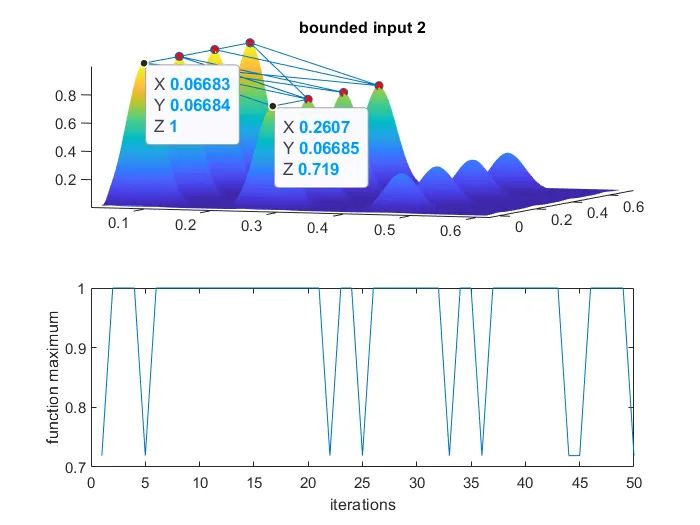
fig. Plot for the optimization_2
Observations:
By adding the bound we have restricted the initial value to be taken by the algorithm which works quite well. Now, we GA has recognized 8 Best fitness values after running the 50 iterations. But the thing to note is that in the above plot only 4 values closely relate to the global maxima, not eight.
Conclusion: we can increase the number of the population by using the default functions of the GA or restrict the bound more to get the exact value.
Optimization_3)
In this for optimization, we have increased the populatoin, for eliminating the selection of the local maxima as clearly can see from the figure above. For this we have used the optimiptions, to increase the size of the optimoptions('ga')
options = optimoptions(options , 'populationsize', 200)
Code for OPtimization_3:
%% Optimization-3 - increasing ga iterations
options = optimoptions('ga')                                          %to select the solver
options = optimoptions(options , 'populationsize', 200)               % to increase the population size
tic
for i = 1:num_iteration
    [inputs , fopt(i)] = ga(@stalgamite_function,2,[],[],[],[],[0;0],[0.6;0.8],[],[],options);
    xopt3(i) = inputs(1);
    yopt3(i) = inputs(2);
end
Study3_Timing = toc
figure
subplot(2,1,1)
hold on
surfc(x,y,-f)
shading interp
plot3(xopt3,yopt3,-fopt,'marker','o','markersize',5,'markerfacecolor','r')
title('Max iterations input 3')
subplot(2,1,2)
plot(-fopt)
xlabel('iterations')
ylabel('function maximum')
Ouput as shown below,
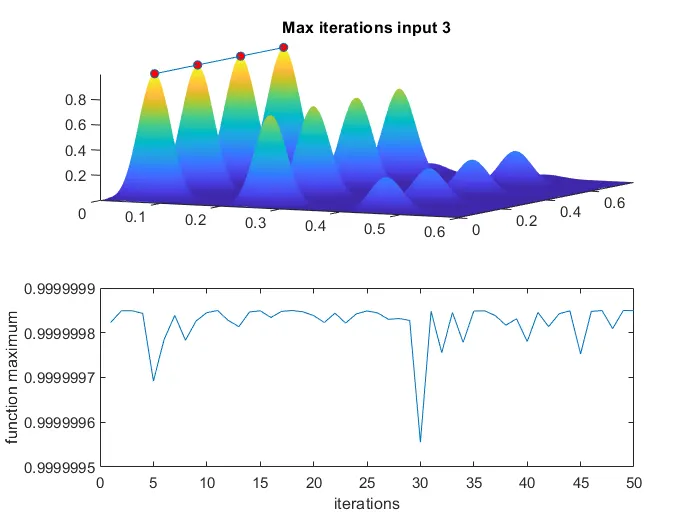
Fig. Plot for optimization_3
Observations: Now, we can easily see the Global maxima of the given Stalagmite function, has same x value for all and maximum function value is nearer to one.
Note: There is no way by which we can guarantee it as the global maxima of the given function.