Unsupervised Learning - Kmeans Week 11 Challenge
1) How does similarity is calculated if data is categorical in nature
Categorical data (also known as nominal data) has been studied for a long time in various contexts. However, computing similarity between categorical data instances is not straightforward owing to the fact that there is no explicit notion of ordering between categorical values. To overcome this problem, several data-driven similarity measures have been proposed for categorical data. The behavior of such measures directly depends on the data. The simplest way to find similarity between two categorical attributes is to assign a similarity of 1 if the values are identical and similarity of 0 if the values are not identical.
Measuring the similarity or distance between two entities is a key step for several data mining and knowledge discovery tasks. The notion of similarity for continuous data is relatively well-understood, but for categorical data, the similarity computation is not straightforward. Several data-driven similarity measures have been proposed in the literature to compute the similarity between two categorical data instances but their relative performance has not been evaluated. In this paper, we study the performance of a variety of similarity measures in the context of a specific data mining task: outlier detection. Results on a variety of data sets show that while no one measure dominates others for all types of problems, some measures are able to have consistently high performance.
the similarity in categorical data is not as direct when it comes to numerical data. the categorical data is first transformed into numerical values and both are standardized to make sense of the similarity and dissimilarities between/among those features. For continuous data sets, the Minkowski Distance is a general method used to compute the distance between two multivariate points. In particular, the Minkowski Distance of order 1 (Manhattan) and order 2 (Euclidean)
are the two most widely used distance measures for continuous data.
The notion of similarity or distance for categorical data is not as straightforward as for continuous data.
The key characteristic of categorical data is that the different values that a categorical attribute takes are
not inherently ordered. Thus, it is not possible to directly compare two different categorical values. The simplest way to find similarity between two categorical attributes is to assign a similarity of 1 if the values are identical and similarity of 0 if the values are not identical.
2) Implement K-means for “Car dataset” and come up with the business insights
import numpy as np
import pandas as pd
import matplotlib.pyplot as plt
from sklearn.cluster import KMeans
df=pd.read_csv('CarPrice_Assignment.csv')
print(df)
car_ID symboling CarName fueltype aspiration \
0         1          3        alfa-romero giulia      gas        std
1         2          3       alfa-romero stelvio      gas        std
2         3          1  alfa-romero Quadrifoglio      gas        std
3         4          2               audi 100 ls      gas        std
4         5          2                audi 100ls      gas        std
..      ...        ...                       ...      ...        ...
200     201         -1           volvo 145e (sw)      gas        std
201     202         -1               volvo 144ea      gas      turbo
202     203         -1               volvo 244dl      gas        std
203     204         -1                 volvo 246   diesel      turbo
204     205         -1               volvo 264gl      gas      turbo

    doornumber      carbody drivewheel enginelocation  wheelbase  ...  \
0          two  convertible        rwd          front       88.6  ...
1          two  convertible        rwd          front       88.6  ...
2          two    hatchback        rwd          front       94.5  ...
3         four        sedan        fwd          front       99.8  ...
4         four        sedan        4wd          front       99.4  ...
..         ...          ...        ...            ...        ...  ...
200       four        sedan        rwd          front      109.1  ...
201       four        sedan        rwd          front      109.1  ...
202       four        sedan        rwd          front      109.1  ...
203       four        sedan        rwd          front      109.1  ...
204       four        sedan        rwd          front      109.1  ...

     enginesize  fuelsystem  boreratio  stroke compressionratio horsepower  \
0           130        mpfi       3.47    2.68              9.0        111
1           130        mpfi       3.47    2.68              9.0        111
2           152        mpfi       2.68    3.47              9.0        154
3           109        mpfi       3.19    3.40             10.0        102
4           136        mpfi       3.19    3.40              8.0        115
..          ...         ...        ...     ...              ...        ...
200         141        mpfi       3.78    3.15              9.5        114
201         141        mpfi       3.78    3.15              8.7        160
202         173        mpfi       3.58    2.87              8.8        134
203         145         idi       3.01    3.40             23.0        106
204         141        mpfi       3.78    3.15              9.5        114

     peakrpm citympg  highwaympg    price
0       5000      21          27  13495.0
1       5000      21          27  16500.0
2       5000      19          26  16500.0
3       5500      24          30  13950.0
4       5500      18          22  17450.0
..       ...     ...         ...      ...
200     5400      23          28  16845.0
201     5300      19          25  19045.0
202     5500      18          23  21485.0
203     4800      26          27  22470.0
204     5400      19          25  22625.0

[205 rows x 26 columns]
print(df.describe())
km=KMeans(n_clusters=3)
print(km)
           car_ID   symboling   wheelbase   carlength    carwidth   carheight  \
count  205.000000  205.000000  205.000000  205.000000  205.000000  205.000000
mean   103.000000    0.834146   98.756585  174.049268   65.907805   53.724878
std     59.322565    1.245307    6.021776   12.337289    2.145204    2.443522
min      1.000000   -2.000000   86.600000  141.100000   60.300000   47.800000
25%     52.000000    0.000000   94.500000  166.300000   64.100000   52.000000
50%    103.000000    1.000000   97.000000  173.200000   65.500000   54.100000
75%    154.000000    2.000000  102.400000  183.100000   66.900000   55.500000
max    205.000000    3.000000  120.900000  208.100000   72.300000   59.800000

        curbweight  enginesize   boreratio      stroke  compressionratio  \
count   205.000000  205.000000  205.000000  205.000000        205.000000
mean   2555.565854  126.907317    3.329756    3.255415         10.142537
std     520.680204   41.642693    0.270844    0.313597          3.972040
min    1488.000000   61.000000    2.540000    2.070000          7.000000
25%    2145.000000   97.000000    3.150000    3.110000          8.600000
50%    2414.000000  120.000000    3.310000    3.290000          9.000000
75%    2935.000000  141.000000    3.580000    3.410000          9.400000
max    4066.000000  326.000000    3.940000    4.170000         23.000000

       horsepower      peakrpm     citympg  highwaympg         price
count  205.000000   205.000000  205.000000  205.000000    205.000000
mean   104.117073  5125.121951   25.219512   30.751220  13276.710571
std     39.544167   476.985643    6.542142    6.886443   7988.852332
min     48.000000  4150.000000   13.000000   16.000000   5118.000000
25%     70.000000  4800.000000   19.000000   25.000000   7788.000000
50%     95.000000  5200.000000   24.000000   30.000000  10295.000000
75%    116.000000  5500.000000   30.000000   34.000000  16503.000000
max    288.000000  6600.000000   49.000000   54.000000  45400.000000
KMeans(n_clusters=3)
y=km.fit_predict(df[["citympg","price"]])
print(y)
[2 2 2 2 2 2 2 2 2 2 2 2 2 2 2 1 1 1 0 0 0 0 0 0 0 0 0 0 0 2 0 0 0 0 0 0 0
 0 0 0 0 2 0 0 0 0 0 1 1 1 0 0 0 0 0 0 0 2 2 0 0 0 0 0 0 2 2 2 1 1 1 1 1 1
 1 2 0 0 0 0 0 0 0 2 2 0 0 0 0 0 0 0 0 0 0 0 0 0 0 0 0 2 2 2 2 2 2 0 2 0 2
 2 2 2 2 2 2 2 0 0 0 0 0 0 2 2 1 1 1 1 0 0 0 0 2 2 2 2 0 0 0 0 0 0 0 0 0 0
 0 0 0 0 0 0 0 0 0 0 0 0 0 0 0 0 0 0 0 0 0 0 0 0 2 0 0 0 0 0 2 2 2 2 0 0 0
 0 0 0 0 0 0 2 2 0 2 2 2 2 2 2 2 2 2 2 2]
df["cluster"]=y
print(df)
df0=df[df.cluster==0]
df1=df[df.cluster==1]
df2=df[df.cluster==2]
print(df0,df1,df2)
car_ID symboling CarName fueltype aspiration \
0 1 3 alfa-romero giulia gas std
1 2 3 alfa-romero stelvio gas std
2 3 1 alfa-romero Quadrifoglio gas std
3 4 2 audi 100 ls gas std
4 5 2 audi 100ls gas std
.. ... ... ... ... ...
200 201 -1 volvo 145e (sw) gas std
201 202 -1 volvo 144ea gas turbo
202 203 -1 volvo 244dl gas std
203 204 -1 volvo 246 diesel turbo
204 205 -1 volvo 264gl gas turbo
doornumber carbody drivewheel enginelocation wheelbase ... \
0 two convertible rwd front 88.6 ...
1 two convertible rwd front 88.6 ...
2 two hatchback rwd front 94.5 ...
3 four sedan fwd front 99.8 ...
4 four sedan 4wd front 99.4 ...
.. ... ... ... ... ... ...
200 four sedan rwd front 109.1 ...
201 four sedan rwd front 109.1 ...
202 four sedan rwd front 109.1 ...
203 four sedan rwd front 109.1 ...
204 four sedan rwd front 109.1 ...
fuelsystem boreratio stroke compressionratio horsepower peakrpm \
0 mpfi 3.47 2.68 9.0 111 5000
1 mpfi 3.47 2.68 9.0 111 5000
2 mpfi 2.68 3.47 9.0 154 5000
3 mpfi 3.19 3.40 10.0 102 5500
4 mpfi 3.19 3.40 8.0 115 5500
.. ... ... ... ... ... ...
200 mpfi 3.78 3.15 9.5 114 5400
201 mpfi 3.78 3.15 8.7 160 5300
202 mpfi 3.58 2.87 8.8 134 5500
203 idi 3.01 3.40 23.0 106 4800
204 mpfi 3.78 3.15 9.5 114 5400
citympg highwaympg price cluster
0 21 27 13495.0 2
1 21 27 16500.0 2
2 19 26 16500.0 2
3 24 30 13950.0 2
4 18 22 17450.0 2
.. ... ... ... ...
200 23 28 16845.0 2
201 19 25 19045.0 2
202 18 23 21485.0 2
203 26 27 22470.0 2
204 19 25 22625.0 2
[205 rows x 27 columns]
car_ID symboling CarName fueltype aspiration \
18 19 2 chevrolet impala gas std
19 20 1 chevrolet monte carlo gas std
20 21 0 chevrolet vega 2300 gas std
21 22 1 dodge rampage gas std
22 23 1 dodge challenger se gas std
.. ... ... ... ... ...
187 188 2 volkswagen super beetle diesel turbo
188 189 2 volkswagen dasher gas std
189 190 3 vw dasher gas std
190 191 3 vw rabbit gas std
193 194 0 volkswagen dasher gas std
doornumber carbody drivewheel enginelocation wheelbase ... \
18 two hatchback fwd front 88.4 ...
19 two hatchback fwd front 94.5 ...
20 four sedan fwd front 94.5 ...
21 two hatchback fwd front 93.7 ...
22 two hatchback fwd front 93.7 ...
.. ... ... ... ... ... ...
187 four sedan fwd front 97.3 ...
188 four sedan fwd front 97.3 ...
189 two convertible fwd front 94.5 ...
190 two hatchback fwd front 94.5 ...
193 four wagon fwd front 100.4 ...
fuelsystem boreratio stroke compressionratio horsepower peakrpm \
18 2bbl 2.91 3.03 9.50 48 5100
19 2bbl 3.03 3.11 9.60 70 5400
20 2bbl 3.03 3.11 9.60 70 5400
21 2bbl 2.97 3.23 9.41 68 5500
22 2bbl 2.97 3.23 9.40 68 5500
.. ... ... ... ... ... ...
187 idi 3.01 3.40 23.00 68 4500
188 mpfi 3.19 3.40 10.00 100 5500
189 mpfi 3.19 3.40 8.50 90 5500
190 mpfi 3.19 3.40 8.50 90 5500
193 mpfi 3.19 3.40 9.00 88 5500
citympg highwaympg price cluster
18 47 53 5151.0 0
19 38 43 6295.0 0
20 38 43 6575.0 0
21 37 41 5572.0 0
22 31 38 6377.0 0
.. ... ... ... ...
187 37 42 9495.0 0
188 26 32 9995.0 0
189 24 29 11595.0 0
190 24 29 9980.0 0
193 25 31 12290.0 0
[124 rows x 27 columns] car_ID symboling CarName fueltype aspiration \
15 16 0 bmw x4 gas std
16 17 0 bmw x5 gas std
17 18 0 bmw x3 gas std
47 48 0 jaguar xj gas std
48 49 0 jaguar xf gas std
49 50 0 jaguar xk gas std
68 69 -1 buick century luxus (sw) diesel turbo
69 70 0 buick century diesel turbo
70 71 -1 buick skyhawk diesel turbo
71 72 -1 buick opel isuzu deluxe gas std
72 73 3 buick skylark gas std
73 74 0 buick century special gas std
74 75 1 buick regal sport coupe (turbo) gas std
126 127 3 porcshce panamera gas std
127 128 3 porsche cayenne gas std
128 129 3 porsche boxter gas std
129 130 1 porsche cayenne gas std
doornumber carbody drivewheel enginelocation wheelbase ... \
15 four sedan rwd front 103.5 ...
16 two sedan rwd front 103.5 ...
17 four sedan rwd front 110.0 ...
47 four sedan rwd front 113.0 ...
48 four sedan rwd front 113.0 ...
49 two sedan rwd front 102.0 ...
68 four wagon rwd front 110.0 ...
69 two hardtop rwd front 106.7 ...
70 four sedan rwd front 115.6 ...
71 four sedan rwd front 115.6 ...
72 two convertible rwd front 96.6 ...
73 four sedan rwd front 120.9 ...
74 two hardtop rwd front 112.0 ...
126 two hardtop rwd rear 89.5 ...
127 two hardtop rwd rear 89.5 ...
128 two convertible rwd rear 89.5 ...
129 two hatchback rwd front 98.4 ...
fuelsystem boreratio stroke compressionratio horsepower peakrpm \
15 mpfi 3.62 3.39 8.0 182 5400
16 mpfi 3.62 3.39 8.0 182 5400
17 mpfi 3.62 3.39 8.0 182 5400
47 mpfi 3.63 4.17 8.1 176 4750
48 mpfi 3.63 4.17 8.1 176 4750
49 mpfi 3.54 2.76 11.5 262 5000
68 idi 3.58 3.64 21.5 123 4350
69 idi 3.58 3.64 21.5 123 4350
70 idi 3.58 3.64 21.5 123 4350
71 mpfi 3.46 3.10 8.3 155 4750
72 mpfi 3.46 3.10 8.3 155 4750
73 mpfi 3.80 3.35 8.0 184 4500
74 mpfi 3.80 3.35 8.0 184 4500
126 mpfi 3.74 2.90 9.5 207 5900
127 mpfi 3.74 2.90 9.5 207 5900
128 mpfi 3.74 2.90 9.5 207 5900
129 mpfi 3.94 3.11 10.0 288 5750
citympg highwaympg price cluster
15 16 22 30760.0 1
16 16 22 41315.0 1
17 15 20 36880.0 1
47 15 19 32250.0 1
48 15 19 35550.0 1
49 13 17 36000.0 1
68 22 25 28248.0 1
69 22 25 28176.0 1
70 22 25 31600.0 1
71 16 18 34184.0 1
72 16 18 35056.0 1
73 14 16 40960.0 1
74 14 16 45400.0 1
126 17 25 32528.0 1
127 17 25 34028.0 1
128 17 25 37028.0 1
129 17 28 31400.5 1
[17 rows x 27 columns] car_ID symboling CarName fueltype aspiration \
0 1 3 alfa-romero giulia gas std
1 2 3 alfa-romero stelvio gas std
2 3 1 alfa-romero Quadrifoglio gas std
3 4 2 audi 100 ls gas std
4 5 2 audi 100ls gas std
.. ... ... ... ... ...
200 201 -1 volvo 145e (sw) gas std
201 202 -1 volvo 144ea gas turbo
202 203 -1 volvo 244dl gas std
203 204 -1 volvo 246 diesel turbo
204 205 -1 volvo 264gl gas turbo
doornumber carbody drivewheel enginelocation wheelbase ... \
0 two convertible rwd front 88.6 ...
1 two convertible rwd front 88.6 ...
2 two hatchback rwd front 94.5 ...
3 four sedan fwd front 99.8 ...
4 four sedan 4wd front 99.4 ...
.. ... ... ... ... ... ...
200 four sedan rwd front 109.1 ...
201 four sedan rwd front 109.1 ...
202 four sedan rwd front 109.1 ...
203 four sedan rwd front 109.1 ...
204 four sedan rwd front 109.1 ...
fuelsystem boreratio stroke compressionratio horsepower peakrpm \
0 mpfi 3.47 2.68 9.0 111 5000
1 mpfi 3.47 2.68 9.0 111 5000
2 mpfi 2.68 3.47 9.0 154 5000
3 mpfi 3.19 3.40 10.0 102 5500
4 mpfi 3.19 3.40 8.0 115 5500
.. ... ... ... ... ... ...
200 mpfi 3.78 3.15 9.5 114 5400
201 mpfi 3.78 3.15 8.7 160 5300
202 mpfi 3.58 2.87 8.8 134 5500
203 idi 3.01 3.40 23.0 106 4800
204 mpfi 3.78 3.15 9.5 114 5400
citympg highwaympg price cluster
0 21 27 13495.0 2
1 21 27 16500.0 2
2 19 26 16500.0 2
3 24 30 13950.0 2
4 18 22 17450.0 2
.. ... ... ... ...
200 23 28 16845.0 2
201 19 25 19045.0 2
202 18 23 21485.0 2
203 26 27 22470.0 2
204 19 25 22625.0 2
[64 rows x 27 columns]
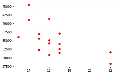
plt.scatter(df1.citympg,df1["price"],color="red")
plt.show()
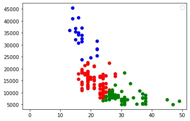
plt.scatter(df0.citympg,df0["price"],color="red")
plt.scatter(df1.citympg,df1["price"],color="blue")
plt.scatter(df2.citympg,df2["price"],color="green")
plt.scatter(km.cluster_centers_[:,0],km.cluster_centers_[:,1],color="purple",marker="")
plt.legend()
plt.show()
def minmax(col):
for i in range(0,len(col)):
new_value=(float(col[i])-float(min(col)))/(float(max(col))-float(min(col)))
ex.append(new_value)
ex=[]
minmax(df.citympg)
df["city_mpg1"]=ex
print(df)
     car_ID  symboling                   CarName fueltype aspiration  \
0         1          3        alfa-romero giulia      gas        std
1         2          3       alfa-romero stelvio      gas        std
2         3          1  alfa-romero Quadrifoglio      gas        std
3         4          2               audi 100 ls      gas        std
4         5          2                audi 100ls      gas        std
..      ...        ...                       ...      ...        ...
200     201         -1           volvo 145e (sw)      gas        std
201     202         -1               volvo 144ea      gas      turbo
202     203         -1               volvo 244dl      gas        std
203     204         -1                 volvo 246   diesel      turbo
204     205         -1               volvo 264gl      gas      turbo

    doornumber      carbody drivewheel enginelocation  wheelbase  ...  \
0          two  convertible        rwd          front       88.6  ...
1          two  convertible        rwd          front       88.6  ...
2          two    hatchback        rwd          front       94.5  ...
3         four        sedan        fwd          front       99.8  ...
4         four        sedan        4wd          front       99.4  ...
..         ...          ...        ...            ...        ...  ...
200       four        sedan        rwd          front      109.1  ...
201       four        sedan        rwd          front      109.1  ...
202       four        sedan        rwd          front      109.1  ...
203       four        sedan        rwd          front      109.1  ...
204       four        sedan        rwd          front      109.1  ...

     boreratio  stroke  compressionratio  horsepower peakrpm citympg  \
0         3.47    2.68               9.0         111    5000      21
1         3.47    2.68               9.0         111    5000      21
2         2.68    3.47               9.0         154    5000      19
3         3.19    3.40              10.0         102    5500      24
4         3.19    3.40               8.0         115    5500      18
..         ...     ...               ...         ...     ...     ...
200       3.78    3.15               9.5         114    5400      23
201       3.78    3.15               8.7         160    5300      19
202       3.58    2.87               8.8         134    5500      18
203       3.01    3.40              23.0         106    4800      26
204       3.78    3.15               9.5         114    5400      19

     highwaympg    price  cluster  city_mpg1
0            27  13495.0        2   0.222222
1            27  16500.0        2   0.222222
2            26  16500.0        2   0.166667
3            30  13950.0        2   0.305556
4            22  17450.0        2   0.138889
..          ...      ...      ...        ...
200          28  16845.0        2   0.277778
201          25  19045.0        2   0.166667
202          23  21485.0        2   0.138889
203          27  22470.0        2   0.361111
204          25  22625.0        2   0.166667

[205 rows x 28 columns]
ex=[]
minmax(df["price"])
df["new_price"]=ex
print(df)
     car_ID  symboling                   CarName fueltype aspiration  \
0         1          3        alfa-romero giulia      gas        std
1         2          3       alfa-romero stelvio      gas        std
2         3          1  alfa-romero Quadrifoglio      gas        std
3         4          2               audi 100 ls      gas        std
4         5          2                audi 100ls      gas        std
..      ...        ...                       ...      ...        ...
200     201         -1           volvo 145e (sw)      gas        std
201     202         -1               volvo 144ea      gas      turbo
202     203         -1               volvo 244dl      gas        std
203     204         -1                 volvo 246   diesel      turbo
204     205         -1               volvo 264gl      gas      turbo

    doornumber      carbody drivewheel enginelocation  wheelbase  ...  stroke  \
0          two  convertible        rwd          front       88.6  ...    2.68
1          two  convertible        rwd          front       88.6  ...    2.68
2          two    hatchback        rwd          front       94.5  ...    3.47
3         four        sedan        fwd          front       99.8  ...    3.40
4         four        sedan        4wd          front       99.4  ...    3.40
..         ...          ...        ...            ...        ...  ...     ...
200       four        sedan        rwd          front      109.1  ...    3.15
201       four        sedan        rwd          front      109.1  ...    3.15
202       four        sedan        rwd          front      109.1  ...    2.87
203       four        sedan        rwd          front      109.1  ...    3.40
204       four        sedan        rwd          front      109.1  ...    3.15

     compressionratio  horsepower  peakrpm citympg highwaympg    price  \
0                 9.0         111     5000      21         27  13495.0
1                 9.0         111     5000      21         27  16500.0
2                 9.0         154     5000      19         26  16500.0
3                10.0         102     5500      24         30  13950.0
4                 8.0         115     5500      18         22  17450.0
..                ...         ...      ...     ...        ...      ...
200               9.5         114     5400      23         28  16845.0
201               8.7         160     5300      19         25  19045.0
202               8.8         134     5500      18         23  21485.0
203              23.0         106     4800      26         27  22470.0
204               9.5         114     5400      19         25  22625.0

    cluster  city_mpg1  new_price
0         2   0.222222   0.207959
1         2   0.222222   0.282558
2         2   0.166667   0.282558
3         2   0.305556   0.219254
4         2   0.138889   0.306142
..      ...        ...        ...
200       2   0.277778   0.291123
201       2   0.166667   0.345738
202       2   0.138889   0.406311
203       2   0.361111   0.430763
204       2   0.166667   0.434611

[205 rows x 29 columns]
km=KMeans(n_clusters=3)
print(km)
KMeans(n_clusters=3)
y_new=km.fit_predict(df[["city_mpg1","new_price"]])
df["cluster_minmax"]=y_new
print(df)
     car_ID  symboling                   CarName fueltype aspiration  \
0         1          3        alfa-romero giulia      gas        std
1         2          3       alfa-romero stelvio      gas        std
2         3          1  alfa-romero Quadrifoglio      gas        std
3         4          2               audi 100 ls      gas        std
4         5          2                audi 100ls      gas        std
..      ...        ...                       ...      ...        ...
200     201         -1           volvo 145e (sw)      gas        std
201     202         -1               volvo 144ea      gas      turbo
202     203         -1               volvo 244dl      gas        std
203     204         -1                 volvo 246   diesel      turbo
204     205         -1               volvo 264gl      gas      turbo

    doornumber      carbody drivewheel enginelocation  wheelbase  ...  \
0          two  convertible        rwd          front       88.6  ...
1          two  convertible        rwd          front       88.6  ...
2          two    hatchback        rwd          front       94.5  ...
3         four        sedan        fwd          front       99.8  ...
4         four        sedan        4wd          front       99.4  ...
..         ...          ...        ...            ...        ...  ...
200       four        sedan        rwd          front      109.1  ...
201       four        sedan        rwd          front      109.1  ...
202       four        sedan        rwd          front      109.1  ...
203       four        sedan        rwd          front      109.1  ...
204       four        sedan        rwd          front      109.1  ...

     compressionratio  horsepower  peakrpm  citympg highwaympg    price  \
0                 9.0         111     5000       21         27  13495.0
1                 9.0         111     5000       21         27  16500.0
2                 9.0         154     5000       19         26  16500.0
3                10.0         102     5500       24         30  13950.0
4                 8.0         115     5500       18         22  17450.0
..                ...         ...      ...      ...        ...      ...
200               9.5         114     5400       23         28  16845.0
201               8.7         160     5300       19         25  19045.0
202               8.8         134     5500       18         23  21485.0
203              23.0         106     4800       26         27  22470.0
204               9.5         114     5400       19         25  22625.0

     cluster city_mpg1  new_price  cluster_minmax
0          2  0.222222   0.207959               0
1          2  0.222222   0.282558               0
2          2  0.166667   0.282558               0
3          2  0.305556   0.219254               0
4          2  0.138889   0.306142               0
..       ...       ...        ...             ...
200        2  0.277778   0.291123               0
201        2  0.166667   0.345738               0
202        2  0.138889   0.406311               0
203        2  0.361111   0.430763               0
204        2  0.166667   0.434611               0

[205 rows x 30 columns]
df0=df[df.cluster_minmax==0]
df1=df[df.cluster_minmax==1]
df2=df[df.cluster_minmax==2]
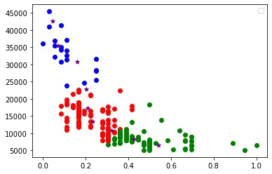
plt.scatter(df0.city_mpg1,df0["price"],color="red")
plt.scatter(df1.city_mpg1,df1["price"],color="blue")
plt.scatter(df2.city_mpg1,df2["price"],color="green")
print(km.cluster_centers_)
print(km.algorithm)
plt.scatter(km.cluster_centers_[:,0],km.cluster_centers_[:,1],color="purple",marker="*")
plt.legend()
plt.show()
[[4.25736961e-01 8.44108163e+03]
 [1.58730159e-01 3.07089286e+04]
 [2.09104938e-01 1.72513380e+04]
 [4.62962963e-02 4.25583333e+04]
 [2.30676329e-01 1.35170435e+04]
 [2.03703704e-01 2.27405556e+04]
 [7.14285714e-02 3.55322857e+04]
 [5.41343669e-01 6.49518605e+03]
 [3.22420635e-01 1.07446786e+04]]
auto
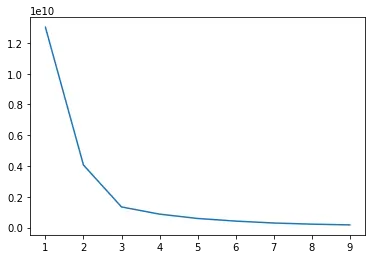
# elbow curve
k_range =range(1,10)
sse=[]
for k in k_range:
km=KMeans(n_clusters=k)
km.fit(df[["city_mpg1","price"]])
sse.append(km.inertia_)
print(sse)
plt.plot(k_range,sse)
plt.show()
[13019639368.730158, 4066798748.743803, 1341589671.6069074, 874350217.9278326, 592651809.056312, 421922997.9901843, 297527096.07242996, 223270865.44694558, 174100038.8407037]
import seaborn as sns
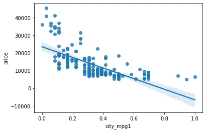
sns.regplot(x="city_mpg1", y="price", data=df)
plt.show()