Understanding the linear system
Aim:
To understand the linear system by finding the eigen values and spectral radius of the given system of matrices.
Objectives:
- To understanding the concept of eigen values and spectral radius.
- To understand how it affects the convergence of the solution.
- To understanding the concept of diagonal dominance.
- To solve the system of matrices by jacobi, gauss seidel and successive over relaxation iterative methods.
- To find the eigen value and spectral radius of the iteration matrix.
Inputs:
The system of matrices to solve are,
Coefficient Matrix, A=[5 1 2 ; -3 9 4; 1 2 -7]
Solution Matrix, X=[x1;x2;x3]
Residual Matrix, B=[10 -14 33]
Eigen values:
The eigen values are the special set of scalar values associated with the linear system solving. The determination of eigen values can be used in various applications. The eigen values plays a vital role in the stability analysis of the linear system. It also helps to find the nature of rotating bodies and small oscillations in the vibrating bodies.
Spectral radius:
The spectral radius is defined as the largest absolute value of the eigen value of the system of matrices. The spectral radius for the finite graph of the finite graph is the maximum or largest eigen values of the adjacency matrix.
Diagonal dominance:
The diagonal dominance is one of the important properties of the matices. A square matrix is said to be diagonally dominant if the magnitude of the diagonal entry in a row is larger than or equal to the sum of the magnitude of the other elements in each row of the matrix.
Iterative methods for solving:
There are three iterative methods available for solving the linear system of matrices. They are,
- Jacobi method
- Gauss seidel method
- Successive over relaxation method
Generally, the given system of matrices can be written as,
A=[5 1 2 ; -3 9 4; 1 2 -7]
X=[x1;x2;x3]
B=[10 -14 33]
==> AX = B
so from this we can find X by,
`X = A^-1*B`
For jacobi method,
The jacobi method is one of the iterative methods for solving governing equation. The discretized equation is solved by assuming some values for the intial solution. The solving process took place till the converged results are obtained. Once a final value is obtained in one iteration, the values are changed by the values obtained in the previous iteration. So the new x value can be obtained as,
x_new = (-(inv(D)*(LTM+UTM))*x_old)+(B*inv(D))
and the eigen value of the system of matrices can be obatined using the formula given below in the jacobi iterative method,
T_jacobi = inv(D)*(LTM+UTM), the eigen value of the T_jacobi will give the eigen values of the system of matrices.
where,
inv(D) is the inversion of Diagonal matrix,
LTM is the Lower Triangular Matrix,
UTM is the Upper Triangular Matrix.
For gauss seidel method,
The gauss seidel method is a type of iterative solver in which the values of the unknowns are assigned initially to get the intial solution as done in jacobi method. The main difference is once a value for an unknown is found, this value is used to get the another value in a same iteration under gauss seidel method. The jacobi method is done with a set of values for one complete iteration. There is not any updation of values occur in jacobi method. So the new x value in gauss seidel can be updated as,
x_new = (-(inv(D+LTM)*(UTM))*x_old)+(B*inv(D+LTM))
and the eigen value of the system of matrices can be obatined using the formula given below in the gauss seidel iterative method,
T_GaussSeidel = (LTM+D)^-1*(-UTM), the eigen value of the T_GaussSeidel will give the eigen values of the system of matrices.
where,
inv(D) is the inversion of Diagonal matrix,
LTM is the Lower Triangular Matrix,
UTM is the Upper Triangular Matrix.
For SOR method,
The successive over relaxation method is an effective iterative solver. The SOR method uses either the solution obtained from jacobi method or from gauss seidel method. In additional to it, the relaxation factor(`omega`) is took in consider in case of SOR method.
Generally, In SOR --> `T_(i,j)=(1-omega)T_(old)+omega*`(Final equation of either gauss seidel or jacobi method). So the new x value in gauss seidel can be updated as,
x_new = -(inv(D+omega*LTM)*((1-omega)*LTM+UTM)*x_old)+(B*inv(D+omega*LTM))
and the eigen value of the system of matrices can be obatined using the formula given below in the SOR iterative method,
T_SOR = (LTM+(1/omega)*D)^-1*(((1/omega)*D)-D-UTM), the eigen value of the T_SOR will give the eigen values of the system of matrices.
where,
inv(D) is the inversion of Diagonal matrix,
LTM is the Lower Triangular Matrix,
UTM is the Upper Triangular Matrix.
Code:
clear all
close all
clc

%Matrices to solve
%Coefficient Matrix

A = [5 1 2 ; -3 9 4; 1 2 -7];

%Residual Matrix

B = [10 -14 33];

%Matrix Decomposition of A
%Diagonal matrix
D = [5 0 0 ; 0 9 0 ; 0 0 -7];

%Lower triangular matrix
LTM = [0 0 0;-3 0 0;1 2 0];

%Upper traingular matrix
UTM = [0 1 2;0 0 4;0 0 0];

%Magnification factor
m = linspace(0.5,5,10);
x_actual = B*inv(A);

%Selecting the iterative solver
Iterative_solver = 3;

%Omega for SOR method
omega = 0.9;


if Iterative_solver == 1
    D_old = D;
    tic
    for i = 1:length(m)
        D = m(i)*D_old;
        l = length(B);
        x_old = zeros(l,1);
        error = 9e9;
        tolerance = 1e-3;

        T_jacobi = inv(D)*(LTM+UTM);

        iter(i)=1;
        while(error > tolerance)

            x_new = (-(inv(D)*(LTM+UTM))*x_old)+(B*inv(D));
            error = max(abs(x_new-x_old));
            x_old = x_new;
            iter(i) = iter(i) + 1;
        end
        x = x_new;

        eigen_value = eig(T_jacobi);
        spectral_radius(i) = max(real(abs(eigen_value)));

    end
    time = toc;

    %Plotting
    figure(1)
    subplot(2,1,1)
    plot(m,spectral_radius,'b')
    xlabel('Magnification Factor')
    ylabel('Spectral radius')
    title({['jacobi method'];['Magnification factor vs spectral radius plot']})
    hold on
    subplot(2,1,2)
    plot(spectral_radius,iter,'r')
    xlabel('spectral radius')
    ylabel('Number of iteration')
    title({['jacobi method'];['Spectral radius vs no. of iteration plot']})
end


if Iterative_solver == 2
    D_old = D;
    tic
    for i = 1:length(m)
        D = m(i)*D_old;
        l = length(B);
        x_old = zeros(l,1);
        error = 9e9;
        tolerance = 1e-3;

        T_GaussSeidel = (LTM+D)^-1*(-UTM);

        iter(i)=1;
        while(error > tolerance)

            x_new = (-(inv(D+LTM)*(UTM))*x_old)+(B*inv(D+LTM));
            error = max(abs(x_new-x_old));
            x_old = x_new;
            iter(i) = iter(i) + 1;
        end
        x = x_new;

        eigen_value = eig(T_GaussSeidel);
        spectral_radius(i) = max(real(abs(eigen_value)));

    end
    time = toc;

    %Plotting
    figure(1)
    subplot(2,1,1)
    plot(m,spectral_radius,'b')
    xlabel('Magnification Factor')
    ylabel('Spectral radius')
    title({['Gauss seidel method'];['Magnification factor vs spectral radius plot']})
    hold on
    subplot(2,1,2)
    plot(spectral_radius,iter,'r')
    xlabel('spectral radius')
    ylabel('Number of iteration')
    title({['Gauss seidel method'];['Spectral radius vs no. of iteration plot']})
end

if Iterative_solver == 3
    D_old = D;
    tic
    for i = 1:length(m)
        D = m(i)*D_old;
        l = length(B);
        x_old = zeros(l,1);
        error = 9e9;
        tolerance = 1e-3;

        T_SOR = (LTM+(1/omega)*D)^-1*(((1/omega)*D)-D-UTM);

        iter(i)=1;
        while(error > tolerance)

            x_new = -(inv(D+omega*LTM)*((1-omega)*LTM+UTM)*x_old)+(B*inv(D+omega*LTM));
            error = max(abs(x_new-x_old));
            x_old = x_new;
            iter(i) = iter(i) + 1;
        end
        x = x_new;

        eigen_value = eig(T_SOR);
        spectral_radius(i) = max(real(abs(eigen_value)));

    end
    time = toc;

    %Plotting
    figure(1)
    subplot(2,1,1)
    plot(m,spectral_radius,'b')
    xlabel('Magnification Factor')
    ylabel('Spectral radius')
    title({['SOR method'];['Magnification factor vs spectral radius plot']})
    hold on
    subplot(2,1,2)
    plot(spectral_radius,iter,'r')
    xlabel('spectral radius')
    ylabel('Number of iteration')
    title({['SOR method'];['Spectral radius vs no. of iteration plot']})
end
Code explanation:
- Initially, the coefficient and residual matrices are assigned.
- The diagonal, lower triangular and upper triangular matrices from matrix A is obtained.
- Various input values are assigned and the iterative method is also selected.
- With the help of formulae shown above, the eigen values and the spectral radius values are obtained.
- Finally, the spectral radius vs magnification factor plot is obtained.
- And the spectral radius vs number of iterations plot is obtained.
Output plots and values:
1) Jacobi method:
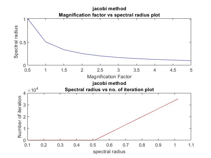
Eigen values - 0.019512590855184 + 0.000000000000000i, -0.009756295427592 + 0.101574120390764i, -0.009756295427592 - 0.101574120390764i
Spectral radius -

Output plot:
2) Gauss seidel method:
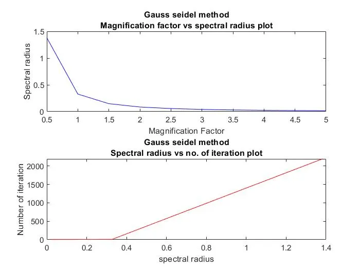
Eigen values - 0, 0.006158623389062, 0.016495131325570.
Spectral radius -

Output Plot:
3) Successive Over Relaxation method:
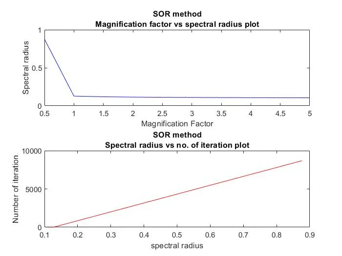
Eigen values - 0.092841312467889 + 0.028586171170884i, 0.092841312467889 - 0.028586171170884i, 0.105969489349938 + 0.000000000000000i.
Spectral radius -

Output plot:
Results and discussions:
- It is observed from the output plot that the spectral radius value increases with decrease in value of the magnification factor.
- So the spectral radius value can be increases by decreasing the magnification factor.
- It is also observed that the number of iteration took by the iterative solvers increases with increase in the spectral radius value.
- When we compared the plots of all the iterative solvers, it is observed that the SOR method took nearly 10,000 iterations for the spectral radius value of nearly 1.
- So the SOR method took less number of iterations to give the converged results for the spectral radius of value 1, when compared with other two iterative plots.
- The number of iterations took by the iterative solvers to get the converged results for the spectral radius value 1 is of the order of Jacobi method > Gauss seidel method > SOR method.
Reference:
https://mathworld.wolfram.com/Eigenvalue.html
https://mathworld.wolfram.com/SpectralRadius.html
https://en.wikipedia.org/wiki/Spectral_radius
https://en.wikipedia.org/wiki/Diagonally_dominant_matrix