Understanding Linear System

Consider the following system of matrices.

Coefficient Matrix, A=[5 1 2 ; -3 9 4; 1 2 -7]

Solution Matrix, X=[x1;x2;x3]

Residual Matrix, B=[10 -14 33]

EXPECTED RESULTS :

• Solve the system of matrices using Jacobi, Gauss-seidel and SOR methods.
• Compute the Iteration Matrix for the above mentioned methods by suitable matrix decomposition techniques taught in the lectures.
• Calculate the Eigen values of the Iteration matrix.
• Calculate the Spectral radius of the Iteration matrix.

Solution:

Eigen Value

Eigenvalues are a special set of scalars associated with a Linear system of equations (i.e., a matrix equation) that are sometimes also known as characteristic roots, characteristic values, proper values, or latent roots.

The determination of the eigenvalues and eigenvectors of a system is extremely important in physics and engineering, where it is equivalent to matrix diagonalization and arises in such common applications as stability analysis, the physics of rotating bodies, and small oscillations of vibrating systems, to name only a few. Each eigenvalue is paired with a corresponding so-called eigenvector (or, in general, a corresponding right eigenvector and a corresponding left eigenvector; there is no analogous distinction between left and right for eigenvalues).

The spectral radius

The spectral radius of a square matrix or a bounded linear operator is the largest absolute value of its eigenvalues.

Jacobi Method

`x^(k+1)=D^(-1)[(-L-U)x^k+B]`

Gauss Seidal Method

`x^(k+1)=(L+D)^-1[-Ux^k+B]`

SOR Method

`x^(k+1) = (L+1/wD)^-1[(1/wD-D-U)x^k+B]`

To understand the linear systems and consistency of iterative techniques we will take a matrix as follows and then determine some parameters which as follow

A=[5 1 2 ; -3 9 4; 1 2 -7]

X=[x1;x2;x3]

B=[10 -14 33]

Function coding:

In function coding, different types of iterative techniques are defined to solve the equation with respect to each technique using a while loop.

basically, while loop solves the equation again and again till we convergence result.

Creating function for Jacobi iteration

% creating a user defined function for jacobi iterative solver
function [jac_iter,x_jac]=jacobi(D,L,U,B)

error=9e9;
tol=1e-4;
x_old=[0;0;0];
jac_iter=1;

%convergence loop
while(error>tol)
    x_jac=(inv(D))*(-L-U)*x_old+(inv(D))*B;
    error=max(abs(x_old-x_jac));
    x_old=x_jac;
    jac_iter=jac_iter+1;
end
end

Creating function for Gauss-Seidel iteration

% creating a user defined function for gauss seidel iterative solver
function [gs_iter,x_gs]=gauss_seidel(D,L,U,B)

error=9e9;
tol=1e-4;
x_old=[0;0;0];
gs_iter=1;

%convergence loop
while(error>tol)
    x_gs=(inv(D+L))*(-U*x_old+B);
    error=max(abs(x_old-x_gs));
    x_old=x_gs;
    gs_iter=gs_iter+1;
end
end

Creating function for Successive Over-Relaxation iteration

% creating a user defined function for sor iterative solver
function [sor_iter,x_sor]=sor(D,L,U,B,w)

error=9e9;
tol=1e-4;
x_old=[0;0;0];
sor_iter=1;

%convergence loop
while(error>tol)
    x_sor=(inv(D-w*L))*((1-w)*D+w*U)*x_old+w*(inv(D-w*L))*B;
    error=max(abs(x_old-x_sor));
    x_old=x_sor;
    sor_iter=sor_iter+1;
end
end

Main coding:

first, matrix A is defined and decomposition of matrix A is done.

Now assign matrix B and magnification factor by using linspace command

Iteration matrix, eigen valuve and spectral radius is calculated fordiffrent iterative techniques

and then we have called the iterative methods and the results are plotted.

% Linear system
clear all
close all
clc

%given co-efficient of matrix A

A = [5 1 2;-3 9 4;1 2 -7]

% decomposition of matrix A
% A = [L+D+U]
L = [0 0 0;3 0 0 ;1 2 0];
D1 = [5 0 0; 0 9 0; 0 0 -7];
U = [0 1 2; 0 0 4; 0 0 0];

%given RHS matrix B
B = [10;-14;33];

%relaxation factor used in sor solver
w = 1.1
%magnification factor
mag_fac = linspace(0.5,5,10)

for i=1:length(mag_fac)
    D = D1*mag_fac(i);
   % to compute iteration matrix for jacobi, gauss seidel and sor(successive
   % over-relaxation)
   T_jac = (inv(D))*(L+U);
   T_gs = (inv(D+L))*U;
   T_sor = (inv(D+w*L))*((1-w)*D-w*U);
   
   % to compute eigen values of iteration matrix for jacobi, gauss seidel and sor
   eigen_value_jac = roots(poly(T_jac));
   eigen_value_gs = roots(poly(T_gs));
   eigen_value_sor = roots(poly(T_sor));
   
   % to compute spectral radius of iteration matrix for jacobi, gauss seidel and sor
   spectral_radius_jac(i) = max(abs(eigen_value_jac));
   spectral_radius_gs(i) = max(abs(eigen_value_gs));
   spectral_radius_sor(i) = max(abs(eigen_value_sor));
  
   %calling iterative method
   [jac_iter(i),x_jac] = jacobi(D,L,U,B);
   [gs_iter(i),x_gs] = gauss_seidel(D,L,U,B);
   [sor_iter(i),x_sor] = sor(D,L,U,B,w);
end 

%plotting for jacobi   
figure(1)
subplot(2,1,1)
hold all
plot(mag_fac,spectral_radius_jac,'-o','markerfacecolor','r','markeredgecolor','r','color','b','linewidth',2)
xlabel('magnification factor','fontsize',10)
ylabel('spectral radius','fontsize',10)
title('Jacobi Method','fontsize',15)
grid on
subplot(2,1,2)
plot(spectral_radius_jac,jac_iter,'color','b','linewidth',2)
xlabel('spectral radius','fontsize',10)
ylabel('Number of iterations','fontsize',10)
grid on

%plotting for gauss seidel
figure(2)
subplot(2,1,1)
hold all
plot(mag_fac,spectral_radius_gs,'-o','markerfacecolor','r','markeredgecolor','r','color','g','linewidth',2)
xlabel('magnification factor','fontsize',10)
ylabel('spectral radius','fontsize',10)
title('Gauss Seidel Method','fontsize',15)
grid on
subplot(2,1,2)
plot(spectral_radius_gs,gs_iter,'color','g','linewidth',2)
xlabel('spectral radius','fontsize',10)
ylabel('Number of iterations','fontsize',10)
grid on

%plotting for sor
figure(3)
subplot(2,1,1)
hold all
plot(mag_fac,spectral_radius_sor,'-o','markerfacecolor','r','markeredgecolor','r','color','y','linewidth',2)
xlabel('magnification factor','fontsize',10)
ylabel('spectral radius','fontsize',10)
title('SOR Method','fontsize',15)
grid on
subplot(2,1,2)
plot(spectral_radius_sor,sor_iter,'color','y','linewidth',2)
xlabel('spectral radius','fontsize',10)
ylabel('Number of iterations','fontsize',10)
grid on

Output:

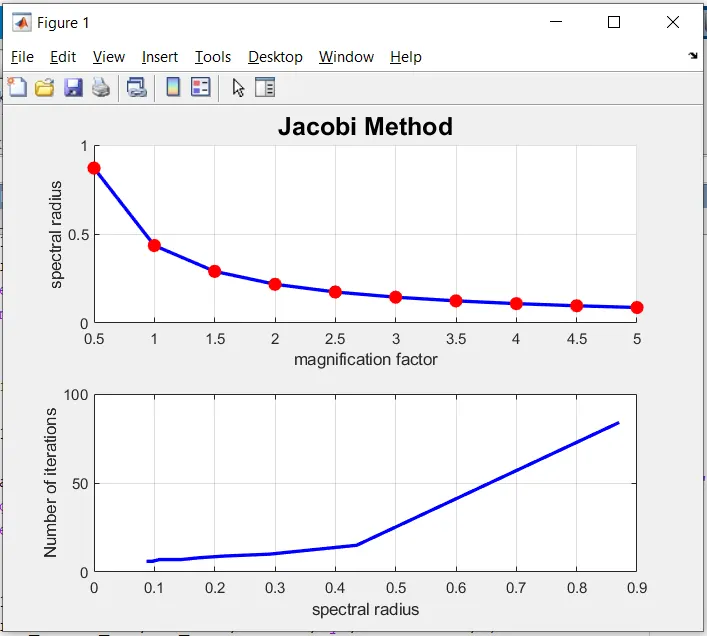
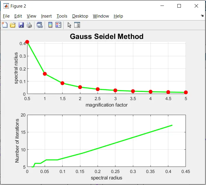
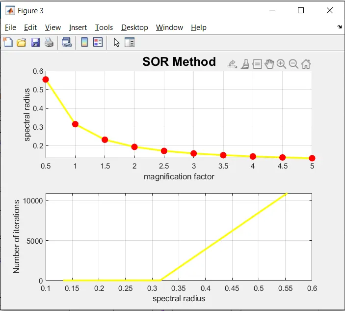
The above plots represent the relation between diagonal magnification vs spectral radius and spectral radius vs the number of iterations.

From the plot, we can say that as diagonal magnification increases the spectral radius decreases, we can say that they are inversely proportional to each other

As the spectral radius increases the number of iterations increases and the result gets converges, hence the spectral radius and number of iterations are directly proportional to each other.

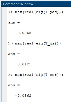
Maximum real eigen values of Jacobi, gauss seidel and sor