TRANSIENT STATE ANALYSIS OF RAYLEIGH TAYLOR INSTABILITY

TRANSIENT STATE ANALYSIS OF RAYLEIGH TAYLOR INSTABILITY

Objective: To perform transient state analysis of Rayleigh Taylor Instability.

INTRODUCTION

In Rayleigh Taylor Instability, when the two fluids the dense fluid at the top and less dense fluid at the bottom the interface between them is unstable because of gravity. As the interface between the fluids collapses the combined potential energy of the fluids decreases and the less dense fluid tries to go upward and the dense fluid downward under the action of gravity. Examples of Rayleigh Taylor waves are interstellar gas, pushed out of the galactic plane by magnetic fields and cosmic rays, becomes RT-unstable if driven beyond its natural scale height. It also occurs at very small scales; e.g., snapping shrimp, which produce most of the ambient noise in subtropical shallow waters throughout the world, produce their sound through collapse of a cavitation bubble, generated by a water jet formed from rapid claw closure; the bubble is destroyed through a Rayleigh-Taylor instability. Similarly, RTI limits the driving pressure in the collapse of acoustically forced bubbles in sonoluminescence phenomena.

PRACTICAL MODEL OF CFD AND MATHEMATICAL MODEL OF RAYLEIGH TAYLOR WAVES

Kelvin–Helmholtz instability

It occurs when the fluids flowing each other have different velocities and the interface between them becomes unstable. The theory also predicts the instability and transition to turbulent flow within fluids of different densities moving at various velocities.

Saffman–Taylor instability

In this the less viscous fluid displaces the unstable interface and form pattern between it and more viscous fluid. In the inverse situation, with the more viscous displacing the other, the interface is stable with no pattern. It is also known as viscous fingering.

Richtmyer–Meshkov instability (RMI)

This occurs when two fluids of different density get impulse at the interaction like a shock wave. The instability develops with minor amplitude deviation. It combines compressible phenomena, such as shock interaction and refraction, with hydrodynamic instability, including nonlinear growth and subsequent transition to turbulence. This instability can be considered the impulsive-acceleration limit of the Rayleigh-Taylor instability.

Plateau–Rayleigh instability

The Plateau–Rayleigh instability, also called as the Rayleigh instability, explains why and how. A liquid jet, initially of constant radius, is falling vertically under gravity. The liquid length increases and reaches a critical value. At this critical value, the jet loses its cylindrical shape as it decomposes into a stream of droplets. It is related to the Rayleigh-Taylor instability and is part of a greater branch of fluid dynamics that deals with fluid thread breakup.

Case 1:

A 2D transient state analysis of Rayleigh Taylor Instability is done using ANSYS FLUENT. Here we have dense fluid at the top and less dense fluid at the bottom the interface is unstable because of gravity. Here the dense fluid is WATER and the less dense fluid is AIR.

Model

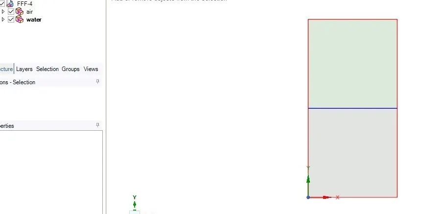
The model was designed in Spaceclaim. Model consists of two squares of 20 mm x 20 mm one above the other. The top surface is water and the bottom surface is air.

Mesh

The model was meshed using ANSYS mesher with element size of 0.5 mm which the BASELINE mesh.

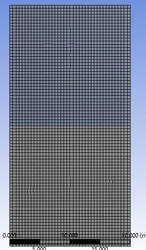
Number of Elements= 3200, Nodes= 3321.

Convergence

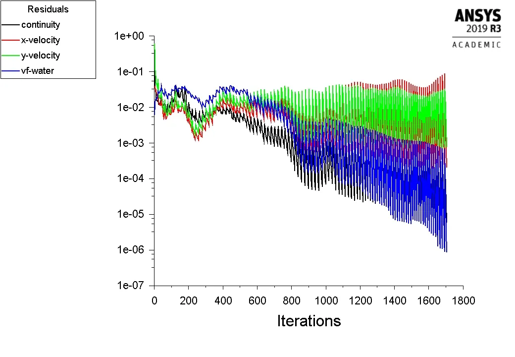
Iteration= 100 were ran and No. of time steps= 0.025 sec. The residual plot is plotted in ANSYS FLUENT shown below.

Result

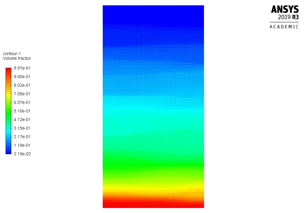
Volume Fraction Contour

Case 2:

A 2D transient state analysis of Rayleigh Taylor Instability is done using ANSYS FLUENT. Here we have dense fluid at the top and less dense fluid at the bottom the interface is unstable because of gravity. Here the dense fluid is WATER and the less dense fluid is AIR.

Model

The model was designed in Spaceclaim. Model consists of two squares of 20 mm x 20 mm one above the other. The top surface is water and the bottom surface is air.

Mesh

The model was meshed using ANSYS mesher with element size of 0.25 mm mesh.

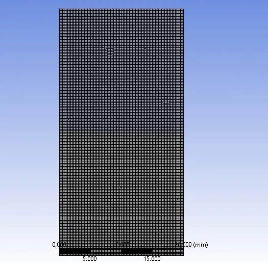
Number of Elements = 12800, Nodes =13041.

Convergence

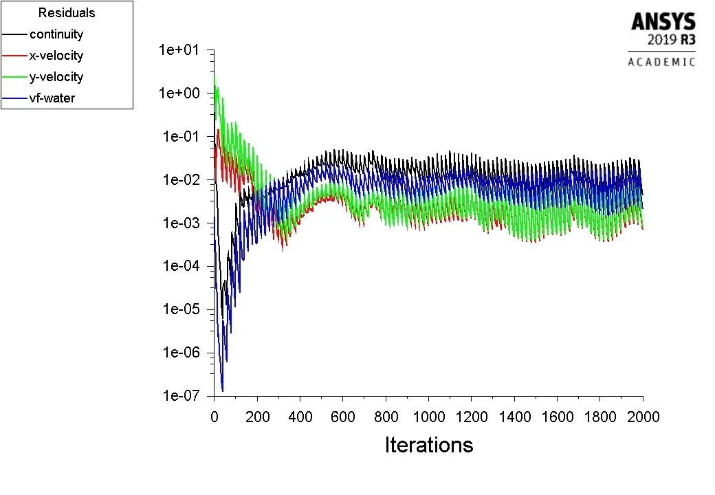
Iteration= 100 were ran and No. of time steps= 0.005 sec. The residual plot is plotted in ANSYS FLUENT shown below.

Result

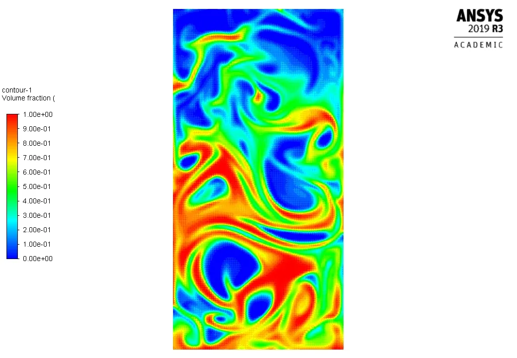
Volume Fraction Contour

Case 3:

A 2D transient state analysis of Rayleigh Taylor Instability is done using ANSYS FLUENT. Here we have dense fluid at the top and less dense fluid at the bottom the interface is unstable because of gravity. Here the dense fluid is WATER and the less dense fluid is AIR.

Model

The model was designed in Spaceclaim. Model consists of two squares of 20 mm x 20 mm one above the other. The top surface is water and the bottom surface is air.

Mesh

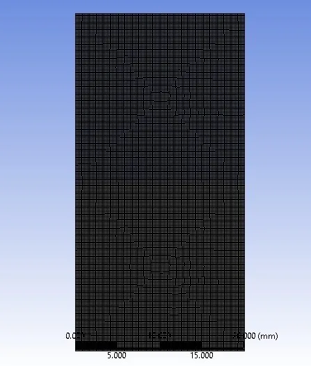
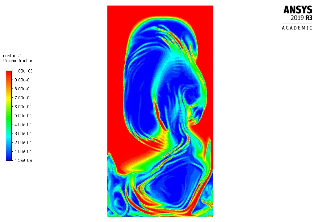
The model was meshed using ANSYS mesher with element size of 0.15 mm mesh. Number of Elements = 35378, Nodes =35778.

Convergence

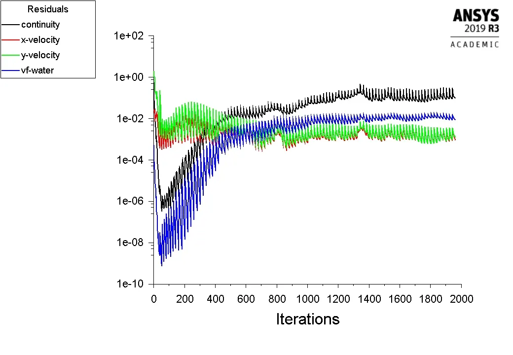
Iteration= 100 were ran and No. of time steps= 0.0025 sec. The residual plot is plotted in ANSYS FLUENT shown below.

Result

Volume Fraction Contour

Case 4:

A 2D transient state analysis of Rayleigh Taylor Instability is done using ANSYS FLUENT. Here we have dense fluid at the top and less dense fluid at the bottom the interface is unstable because of gravity. Here the dense fluid is WATER and the less dense fluid is AIR.

Model

The model was designed in Spaceclaim. Model consists of two squares of 20 mm x 20 mm one above the other. The top surface is water and the bottom surface is air.

Mesh

The model was meshed using ANSYS mesher with element size of 0.1 mm mesh. Number of Elements = 80000, Nodes =80601.

Convergence

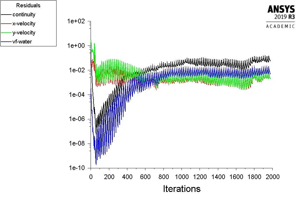
Iteration= 100 were ran and No. of time steps= 0.0025 sec. The residual plot is plotted in ANSYS FLUENT shown below.

Result

Volume Fraction Contour

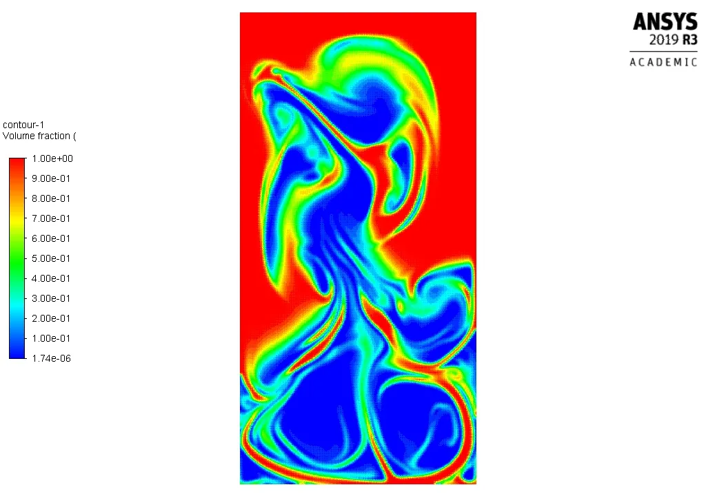
ATWOOD NUMBER

The Atwood number (A) is a dimensionless number in fluid dynamics used in the study of hydrodynamic instabilities in density stratified flows. It is a dimensionless density ratio defined as

A = `(⍴_1-⍴_2 )/(⍴_1+⍴_2)`

Where,

`⍴_1` = density of more dense fluid

`⍴_2`= density of less dense fluid

Density of air= 1.225 kg/m³

Density of water= 1000 kg/m³

Now Atwood number between air and water is

A = `(1000-1.225)/(1000+1.225)` = 0.997

OIL AND WATER

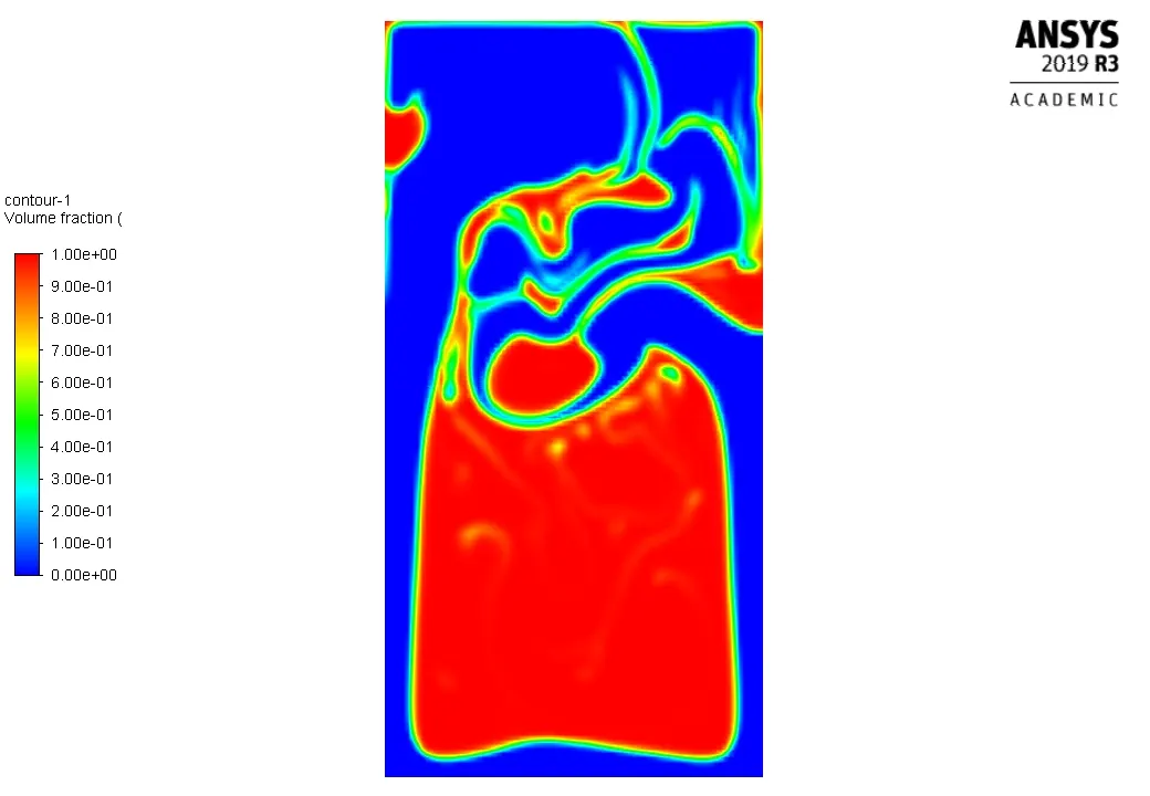
A 2D transient state analysis of Rayleigh Taylor Instability is done using ANSYS FLUENT. Here we have dense fluid at the top and less dense fluid at the bottom the interface is unstable because of gravity. Here the dense fluid is WATER and the less dense fluid is OIL.

Model

The model was designed in Spaceclaim. Model consists of two squares of 20 mm x 20 mm one above the other. The top surface is water and the bottom surface is oil. Oil properties are Density = 400 kg/m³, Dynamic Viscocity = 1.06 kg/m-s.

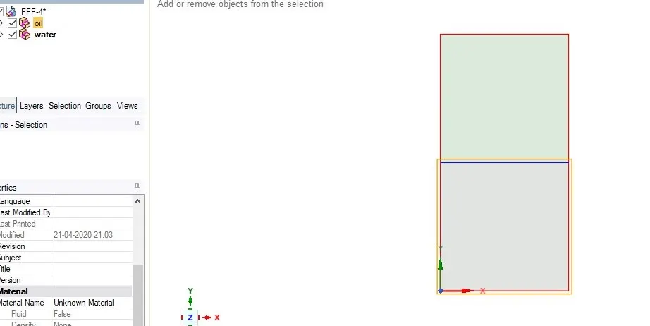
Mesh

The model was meshed using ANSYS mesher with element size of 0.25 mm mesh. Number of Elements = 12800, Nodes =13041.

Convergence

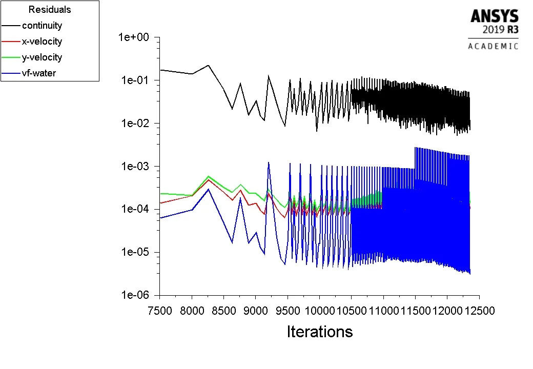
Iteration= 1000 were ran and No. of time steps= 0.0025 sec. The residual plot is plotted in ANSYS FLUENT shown below.

Result

Volume Fraction Contour

ATWOOD NUMBER

Density of oil= 400 kg/m³

Density of water= 1000 kg/m³

Atwood number between air and water is

A = `(1000-400)/(1000+400)` = 0.428

EFFECTS OF ATWOOD NUMBER ON RAYLEIGH TAYLOR INSTABILITY

• Atwood number between air and water interface is 0.428
• Atwood number between oil and water interface is 0.997
• When A<=1 the less dense fluid move into more dense fluid in the form of bubbles of circular cross section. The denser fluid will form spikes and wall or curtains between the bubbles so that the horizontal section will show a honeycomb pattern.
• When A>=0 there is a pattern more like two sets of interpenetrating bubbles.

TRANSIENT ANALYSIS PREFERRED OVER STEADY STATE ANALYSIS

Since we have to get the instability pattern at the interface of two fluids and this happens with time as the steady state analysis is independent of time we consider transient state analysis.

Conclusion

The refinement done in the mesh gives better flow pattern in water and air, also we get results of oil and water interface. This is both happens using Transient state analysis.