To visualize and solve a otto cycle using matlab

Question- To visualize and solve a otto cycle using Matalab.
Theortical Relations/formulaes: Following are the formulaes to solve an otto cycle

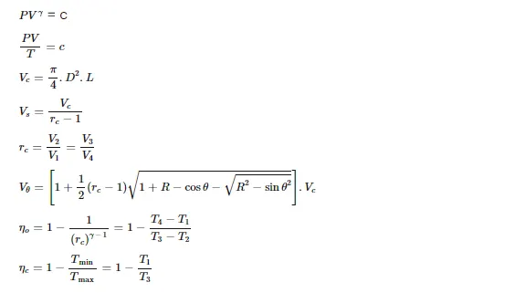
where;

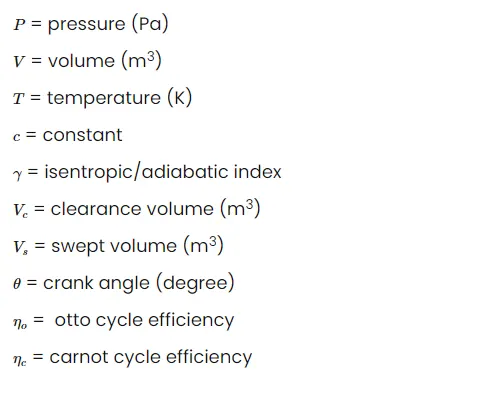
Objective-
1- To Plot P-V diagram of an Otto Cycle.
2- To calculate the thermal efficiency.
3- To study piston kinematics by using of an OttoCycle,as a function in the isentropic processses.

Literature:
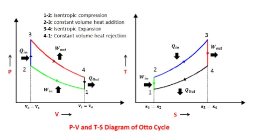
An Otto Cycle is an idealized thermodynamic cycle that describes the functioning of a typical spark ignition piston engine.It is the thermodynamic cycle most commonly found in automobile engines. The processes involved during the cycle is as follows;

Process 1-2: Adiabatic (isentropic) compression of the charge as the piston moves from the bottom
dead centre(BDC) to top dead centre(TDC).

Process 2-3: Constant -volume heat transfer to the working fuel and air mxture from an external source
while the piston is at the top dead centre. This process is intended to represent the ignition of the fuel-air mixture and the subsequent rapid burning

Process 3-4: Adiabatic(isentropic) expansion (power stroke)

Process 4-1: Complete the cycle by a constant- volume process in which heat is rejected from the
air while the piston is at bottom dead centre.

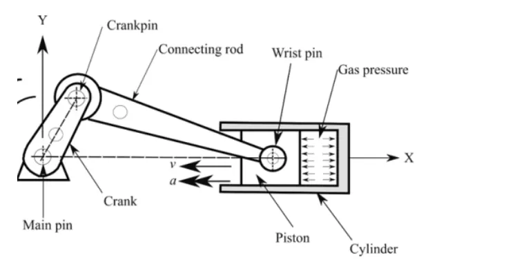
Piston Kinematics: Piston kinematics is the study of the motion of the piston relative to the rotation of the
crankshaft.A reciprocating engine derives its power from the vertical motion of the piston within individual
cyclinders of the engine.The up-down motion of the piston, also known as reciprocating motiion,is converted into rotatory motion by the use of a crankshaft.

Solution:
Procedure:
Step 1- Assign the suitable variables to store the input
parameters of the engine and the state parameter.
Step 2- Calculate swept volume and clearance volume with
the help of given equation.
Step 3- By using the Gas Law and other process relation,
calcualate the thermodynamic data at all state.
Step 4- An array is used to find out the v_comp,p_comp
and v_exp,p_exp.
Step-5 Now efficiency for otto cycle are calculated with
the help of the formulaes.
Step-6 Now the curves are plotted for the processes.
Step-7 Finally all the states point are shown

Code: Below is the Matlab code to plot the P-V diagram
is shown below.

%Program to plot P-V Diagram and calculate the efficiency of otto cycle.
% Inputs:
% p= pressure(pa),v=volume(m^3),t=temperature(k))
gamma = 1.4; %Isentropic Index
cr = 10; % Isentropic or Compression ratio
% Engine Geometric Parametes cr=v1/v2
bore = 0.1; % bore Diameter(m)
stroke = 0.1;%stroke length(m)
con_rod = 0.15;%Connecting Rod length(m)
% State 1
p1 = 101325;
t1 = 350;
%State3
t3 = 1500;
%solution:
% State 1
v_s = (pi/4)*(bore^2)*stroke; % swept volume
v_c = v_s/(cr-1); % Clearnce Volume
v1 = v_c + v_s
% State 2
v2 = v_c;
% p1*v1^gamma = p2*v2^gamma | p2= p1* (v1/v2)^gamma | p2= p1*(cr^gamma)
p2= p1*(cr^gamma);
% p1*v1/t1 = p2*v2/t2 | t2= (p2*v2*t1)/(p1*v1);
t2= (p2*v2*t1)/(p1*v1);
% Parameters during isentropic compression
c1 = p1*v1^gamma;
v_comp = otto_cycle_kinematics(bore,stroke,con_rod,cr,0,180);
p_comp = c1./(v_comp.^gamma);
% State 3;
v3 = v2;
% p2*v2/t2 = p3*v3/t3
p3 = p2*t3/t2;
%Parameters during Isentropic Expansion
c3 = p3*v3^gamma;
v_exp = otto_cycle_kinematics(bore,stroke,con_rod,cr,180,0);
p_exp = c3./(v_exp.^gamma);
% State 4
v4 = v1;
% p3*v3^gamma = p4*v4^gamma| p4 = p3*(v3/v4)^gamma
p4 = p3*(v3/v4)^gamma;
% p3*v3/t3 = p4*v4/t4
t4 = (p4*v4*t3)/(p3*v3);
% Efficiency
otto_eff = (1- ((t4-t1)/(t3-t2)))*100
carnot_eff = (1-(t1/t3))*100
txt = ['Efficiency=',num2str(otto_eff),'%'];

%Plot:
figure(1)
hold on
plot(v_comp,p_comp,'color','m')
plot([v2 v3],[p2 p3],'color','g')
plot(v_exp,p_exp,'color','b')
plot([v1 v4],[p1 p4],'color','k')
plot(v1,p1,'x','color','r')
plot(v2,p2,'x','color','r')
plot(v3,p3,'x','color','r')
plot(v4,p4,'x','color','r')
text(v1,p1,'1','HorizontalAlignment','left','VerticalAlignment','top')
text(v2,p2,'2','HorizontalAlignment','right','VerticalAlignment','top')
text(v3,p3,'3','HorizontalAlignment','right','VerticalAlignment','bottom')
text(v4,p4,'4','HorizontalAlignment','left','VerticalAlignment','bottom')
xlabel('Volume(m^3)')
ylabel('Pressure(Pa)')
axis([0 0.0011 -600000 5500000])
title('P-V diagram of Otto Cycle')
legend('Constant volume heat rejection','Isentropic compression','Constant volume heat addition','Isentropic expansion')
grid on
% End of the program

Output:
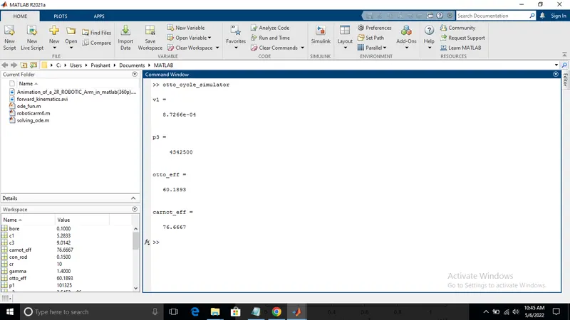
The efficiency for both otto and carnot cycle are calculated and the problem is solved and the image of the command window is attached below.

Plot:
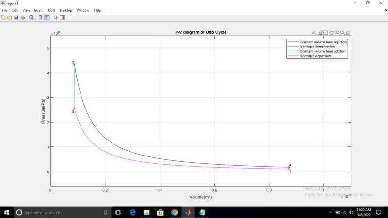
All the four states point are plotted and connected according to their respective thermodynamic process nature as shown below

Function : Below is the function for calcualting the v_comp,p_comp and v_exp,v_exp.
We call the function otto_cycle_kinematics to find the volume trace as a function of crank angle during compression and expansion process.

% Program to calculate Volume with variation in crank angle
function [V] = otto_cycle_kinematics(bore,stroke,con_rod,cr,start_crank,end_crank)
% Inputs
% Engine Geometric Parametes cr=v1/v2
a = stroke/2; % crank pin radius
R=con_rod/a; % crank ratio
% Solution:
v_s = (pi/4)*(bore^2)*stroke; % swept volume
v_c = v_s/(cr-1);
theta = linspace(start_crank,end_crank,100);
term_1 = (cr-1)/2;
term_2 = 1+ R - cosd(theta);
term_3 = (R^2 - sind(theta).^2).^0.5;

V= (1+ term_1*(term_2-term_3)).*v_c; % volume in terms of crank angle

% Plot:

plot(V)
xlabel('Crank angle(deg)')
ylabel('volume(m^3)')
grid on
end
% end of the program

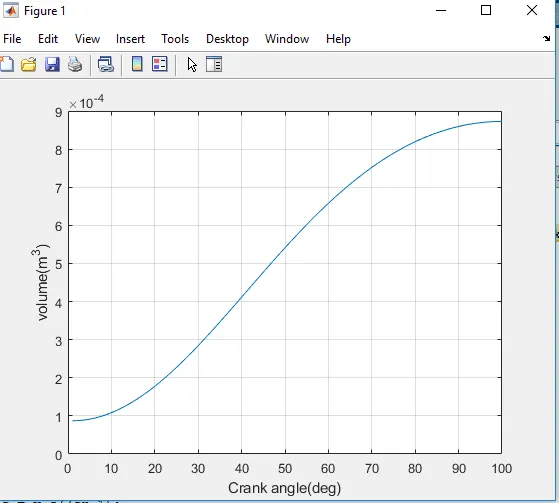
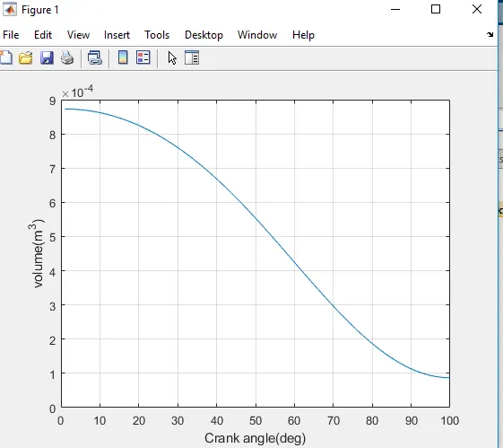
Plot: The variation and nature of volume with crank angle rotation is shown below.

Error- As the complete code is correct and their is no error observed in the program and the command window is also displayed above.

Solution - A function was written which included the crank angle and volume
during the compression and expansion process.Also, seprate plot commands were
given for each state points so that they are displayed according to their
process nature.

Conclusion- From the above results, we can infer that the otto cycle efficiency
is less as comapred to Carnot cycle efficiency .