To determine Thermal Efficiency of Otto Cycle by using Matlab

Aim :-

To determine the thermal efficiency of the otto cycle with pv diagram using matlab.

Governing Equation :-

`PV = NRT`

`〖PV〗^γ = constant`

`(PV)/T = constant`

`μ = 1 -(〖1/(compression ratio))〗^(γ-1)`

`V_s= π/4* 〖D〗^2*l`

`V_c= V_s/(compression ratio-1)`

Objective :-

1. To calculate the thermal efficiency
2. To calaculate the pressure (P), Temperature (T) and Volume (V) at every state points
3. To plot the pv diagram

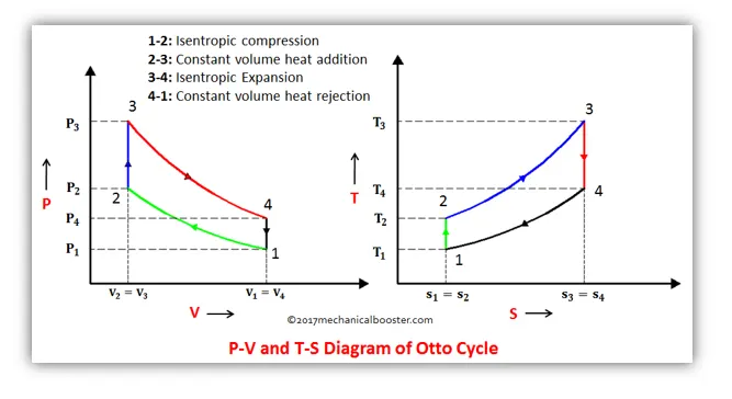
Process of Otto Cycle :-

Process 1-2 :- Isentropic Compression process, where pressure, temperature increases and volume decreases with constant entropy.

Process 2-3 :- Constant Volume heat addition process, where pressure, temperature and entropy increases.

Process 3-4 :- Isentropic expansion process, where pressure, temperature decreases and volume increases with constant entropy.

Process 4-5 :- Constant volume heat rejection process, where pressure, temperature and entropy decreases.

Content Body :-

clear all
close all
clc

%Input
gamma = 1.4
t3 = 2000

%state variable
p1 = 101325;
t1 = 400;

%Engine Geometric Paramater
bore = 0.09;
stroke = 0.11;
con_rod = 0.17;
cr = 15;

%calculating the swept volume and clearance volume
swept_vol = (pi/4)*bore^2*stroke
clear_vol = swept_vol/(cr-1)

v1 = swept_vol + clear_vol;
v2 = clear_vol;

%state variable at state point 2
%p1v1^gamma = p2v2^gamma
%p2 = p1(v1/v2)^gamma = p1*cr^gamma
p2 = p1*cr^gamma

%p1v1/t1 = p2v2/t2 ; t2 = p2*v2*t1/p1*v1
t2 = p2*v2*t1/(p1*v1)

constant_c = p1*v1^gamma;
V_compression = engine_kinamatics(bore,stroke,con_rod,15,180,0)
P_compression = constant_c./V_compression.^gamma;

  %state variable at state point 3
v3 = v2;

%p3v3/t3 = p2v2/t2 ; p3 = p2*v2*t3/(t2*v3)
p3 = p2*v2*t3/(t2*v3)

constant_c = p3*v3^gamma;
V_expansion = engine_kinamatics(bore,stroke,con_rod,15,0,180);
P_expansion = constant_c./V_expansion.^gamma;

% state variable at state point 4
v4 = v1;

%p3v3^gamma = p4v4^gamma ; p4 = p3(v3/v4)^gamma
p4 = p3*(v3/v4)^gamma 

thermal_efficiency = 1-(1/cr)^(gamma-1)

figure(1)
hold on
plot(v1,p1,'*','color','r')
plot(V_compression,P_compression,'color','b','linewidth',1)
plot(v2,p2,'*','color','r')
plot(v3,p3,'*','color','r')
plot(V_expansion,P_expansion,'color','b','linewidth',1)
plot(v4,p4,'*','color','r')
plot([v2 v3],[p2 p3],'color','b','linewidth',1)
plot([v4 v1],[p4 p1],'color','b','linewidth',1)
xlabel('volume')
ylabel('pressure')

​

1. We have initial conditions of state point 1 through which we can calculate P,V and T for all the state points
2. We have used function code to call the function which is used as a template to determine compression volume and expansion volume at each and every point when the piston moves from 0 to 180 degrees and 180 to 0 degrees.
3. While coding I faced an error where my constant ( C ) was undefined to calculate compression pressure at each and every point. So I calculated my constant ( C ) first.
4. Second error I faced was, I copied and pasted compression volume formula to calculate expansion volume, which results that my plots gave only compression volume curve.
5. After re-checking every line, I found my mistake and corrected.

Conclusion :-

Thermal Efficiency is as below.

`μ=0.6615`

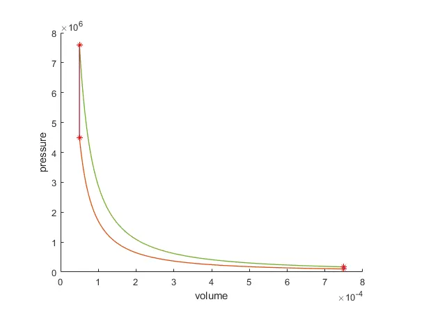
Result :-

Hence we have plotted the PV diagram and calculated the thermal efficiency.