Taylor table method and Matlab code

Q1. Derive the following 4th order approximations of the second-order derivative.

1. Central difference

2. Skewed right-sided difference

3. Skewed left-sided difference

Also, prove that your skewed schemes are fourth-order accurate.

Once you have done this, write a program in Matlab to evaluate the second-order derivative of the analytical function exp(x)*cos(x) and compare it with the 3 numerical approximations that you have derived.

a. Provide a plot that compares the absolute error between the above-mentioned schemes.

b. In your own words, describe why a skewed scheme is useful? What can a skewed scheme do that a CD scheme cannot?

Ans:

Taylor Series: Represents a function as an infinite sumof terms that are calculated from the values of function derivative at a single point

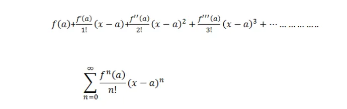
where n! is factorial of n and nth derivative of f is evaluated at a. When a= 0 the above series is called a Maclaurin series.

Aim: To drive Central difference, Skewed right difference, and skewed left difference scheme for fourth order approximation of second order derivative by using Taylor table method of finite difference method.

1. Central difference:

For fourth order approximation, 5 points stencil is selected.

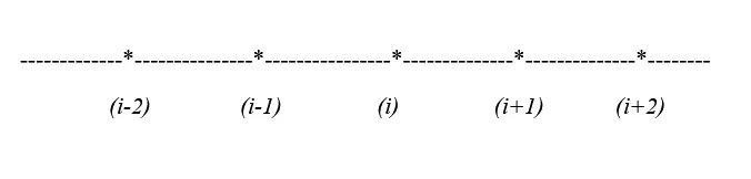
Second order derivative of 4th order approximation for CDS is:

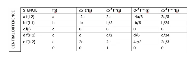
`(del^2f)/(delx^2)= af(i-2) +bf(i-1)+cf(i)+df(i+1)+ef(i+2)`

After simplifying the above equation, following taylor table is obtained:

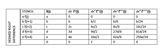
2. Skewed right side difference:

The stencil used in this is :

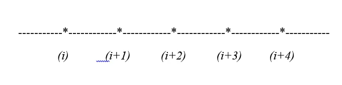
Second order derivative of 4th order approximation for SRSD is:

`(del^2f)/(delx^2)=af(i)+bf(i+1)+cf(i+2)+df(i+3)+ef(i+4)`

After simplifying the above equation, following taylor table is obtained:

3. Skewed left side difference:

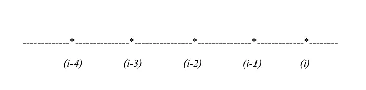
The stencil used in this is :

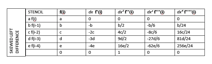
Second order derivative of 4th order approximation for SLSD is:

`(del^2f)/(delx^2)=af(i) + bf(i-1) +cf(i-2)+df(i-3)+ef(i-4)`

After simplifying the above equation, following taylor table is obtained:

Now to solve this, following function in Octave is made along with the main function:

The first function is to calculate the coefficient of central difference and returns the error from the analytical derivative of the given function.

The given function is :

`f(x)=e^x .cos(x)`

Analytical derivative= `-2e^x sin(x)`

A. Central differencing

function out= central_difference(x,dx)
%function given= exp(x)*cos(x)
a= [1 1 1 1 1; -2 -1 0 1 2; 2 0.5 0 0.5 2; -8/6, -1/6, 0, 1/6, 8/6; 16/24, 1/24, 0, 1/24, 16/24 ];
b= [0; 0; 1; 0; 0];
c=inv(a)*b;
%analytical_derivative= -2*sin(x)*exp(x)
analytical_derivative= -2*sin(x)*exp(x);
%error calulation
central_difference_approx=(c(1)*exp(x-2*dx)*cos(x-2*dx)+c(2)*exp(x-dx)*cos(x-dx)+c(3)*exp(x)*cos(x)+c(4)*exp(x+dx)*cos(x+dx)+c(5)*exp(x+2*dx)*cos(x+2*dx))/((dx)^2);
out=abs(central_difference_approx-analytical_derivative);
endfunction

As we can see, the above code calculates the coefficients of the central difference approximation using matrix inversion.

a= -0.083333
b= 1.333333
c= -2.500000
d= 1.333333
e= -0.083333

for `(del^2f)/(delx^2)= af(i-2) +bf(i-1)+cf(i)+df(i+1)+ef(i+2)`

B. Skewed right side difference:

function out= skewed_right_difference(x,dx)
%function given= exp(x)*cos(x)
a=[1 1 1 1 1; 0 1 2 3 4; 0 1/2 4/2 9/2 16/2; 0 1/6 8/6 27/6 64/6; 0 1/24 16/24 81/24 256/24];
b= [0; 0; 1; 0; 0];
c=inv(a)*b;
%analytical_derivative= -2*sin(x)*exp(x)
analytical_derivative= -2*sin(x)*exp(x);
%error calulation
skewed_right_approx=(c(1)*exp(x)*cos(x)+c(2)*exp(x+dx)*cos(x+dx)+c(3)*exp(x+2*dx)*cos(x+2*dx)+c(4)*exp(x+3*dx)*cos(x+3*dx)+c(5)*exp(x+4*dx)*cos(x+4*dx))/((dx)^2);
out=abs(skewed_right_approx-analytical_derivative);
endfunction

From here we get the coefficients:

a= 2.91667
b= -8.66667
c= 9.50000
d= -4.66667
e= 0.91667

for `(del^2f)/(delx^2)=af(i)+bf(i+1)+cf(i+2)+df(i+3)+ef(i+4)`.

C. Skewed left side difference:

function out= skewed_left_difference(x,dx)
%function given= exp(x)*cos(x)
a=[1 1 1 1 1; 0 -1 -2 -3 -4; 0 1/2 4/2 9/2 16/2; 0 -1/6 -8/6 -27/6 -64/6; 0 1/24 16/24 81/24 256/24];
b= [0; 0; 1; 0; 0];
c=inv(a)*b;
%analytical_derivative= -2*sin(x)*exp(x)
analytical_derivative= -2*sin(x)*exp(x);
%error calulation
skewed_left_approx=(c(1)*exp(x)*cos(x)+c(2)*exp(x-dx)*cos(x-dx)+c(3)*exp(x-2*dx)*cos(x-2*dx)+c(4)*exp(x-3*dx)*cos(x-3*dx)+c(5)*exp(x-4*dx)*cos(x-4*dx))/((dx)^2);
out=abs(skewed_left_approx-analytical_derivative);
endfunction

Value of coefficients:

a= 2.91667
b= -8.66667
c= 9.50000
d= -4.66667
e= 0.91667

for `(del^2f)/(delx^2)=af(i) + bf(i-1) +cf(i-2)+df(i-3)+ef(i-4)`.

MAIN PROGRAM:

clear all
close all
clc

%given value of x and range of dx
x=pi/3;
dx=linspace(pi/4,pi/4000,2000);

for i=1:length(dx)
  cd_error(i)=central_difference(x,dx(i));
  sr_error(i)=skewed_right_difference(x,dx(i));
  sl_error(i)=skewed_left_difference(x,dx(i));
endfor
%ploting of the graphs for comparing
figure(1)
loglog(dx,cd_error,'b')
hold on
loglog(dx,sr_error,'r')
hold on
loglog(dx,sl_error,'g')

xlabel('dx')
ylabel('Errors')
legend('central difference','skewed right difference','skewed left difference')

In this code,

1. All the three schemes are called and compared to each oth better understanding.
2. The range of dx is from `pi/4` to `pi/4000`.
3. log graph is used for enlarged scale.

After running the code following result is obtained:

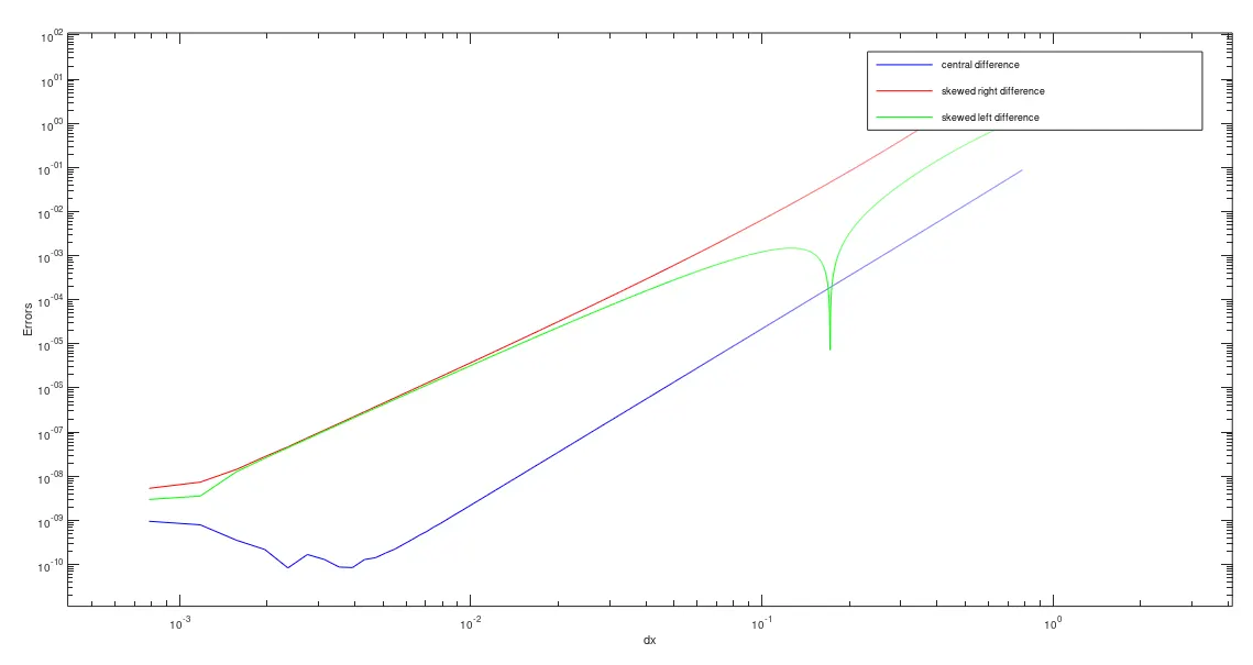
Plot: dx vs Error

From here we can conclude that:

1. Skewed right side difference gives the maximum error at almost every point of the dx.
2. The central difference gives the lowest error and is consistent throughout the range of dx.
3. Skewed left is quite unstable as at some point it gives a lower error value than the central difference and at some point it becomes almost equal to SRS difference.
4. On dropping the value of dx, the value of error also decreases. As they all are a fourth-order approximation, the slope of the curve is almost similar tp each other.

Q2. why a skewed scheme is useful? What can a skewed scheme do that a CD scheme cannot?

As we know that these schemes are used to calculate the derivative of the function at a certain point like in this case it is `pi/3`. This point lies somewhere but not the endpoint/boundary points.

When it comes to calculating the derivative at boundary points, the central difference can't be used. This is because the in central difference data from both sides of the curve is required but at the boundary only one side is available.

To calculate the derivate at boundary points, Skewed right side difference and Skewed left side difference can be used. Sometimes forward difference and the backward difference can also be used but due to lack of higher-order terms, the higher-order approximation can not be calculated.

Although the Central difference gives the least error but when it comes to boundary points, due to lack of neighboring information, skewed schemes are used and gives stable results.