Taylor table method and Matlab code to find the 4th order approximation of second order derivative

Aim:

To derive the 4th order approximation of second-order derivative in three different schemes and to analysed the errors on each schemes.

Objectives:

• To derive the 4th order approximation of the second order derivative for central difference, skewed right-sided difference and skewed left-sided difference schemes.
• To prove that the skewed schemes are fourth-order accurate.
• To write a code in matlab to evaluate the second-order derivative of the analytical function exp(x)*cos(x).
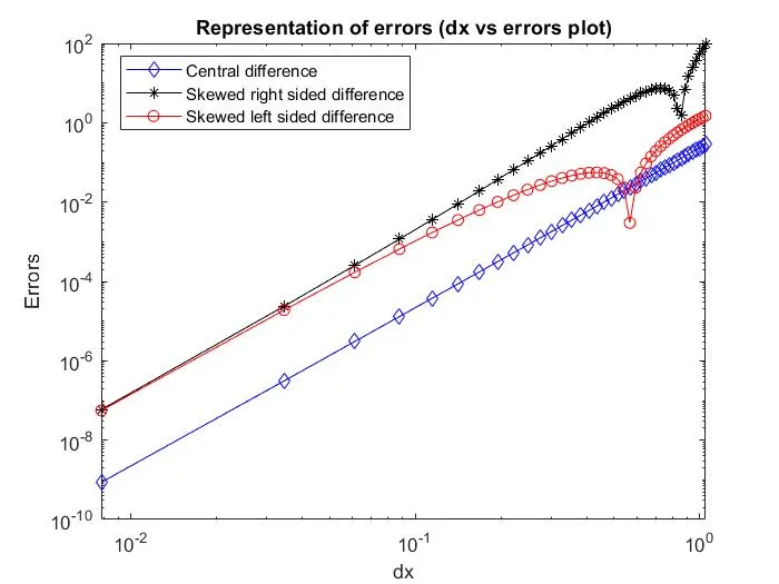
• To represent a plot that compares the absolute error between the three schemes.

Discretization:

Discretization is a process of transferring the function or equation into discrete points. This discretization process helps to convert the partial differential equations into algebraic function. Discretization plays a pivotal role in the computational fluid dynamics domain. There are various methods of discretization,

• Finite element method.
• Finite difference method.
• Finite volume method.

Taylor series and taylor table play a pivotal role in the process of discretization. In finite difference method, based on the information obtained from the reference node three schemes are assigned. They are,

• Central difference scheme
• Skewed right-sided difference
• Skewed left-sided difference

The central difference scheme is a type of scheme in which the reference node is at the centre and the information is obtained from the nodes at both sides of the reference nodes. The amount of nodes considered from the reference node is equal on both the sides so that the central difference scheme is symmetrical. The skewed right-sided difference is a type of scheme in which the discretized points or nodes lies on the right side of the reference node. Similarly, the skewed left-sided difference is a type of scheme in which the discretized points or nodes lies on the left side of the reference node.

Central difference scheme:

The central difference scheme for 4th order approximation of second order derivative is to be calculated. The number of nodes can be calculated from the formula n=(p+q)-1 for central difference scheme. The term 'n' denotes the number of nodes, 'p' denotes the order of derivative and 'q' denotes the order of approximation.

p = 2 (2nd order derivative)

q = 4 (4th order approximation)

n = (p+q)-1

= (2+4)-1

number of nodes = 5

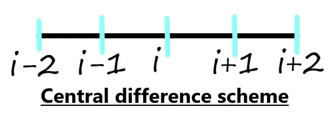
The distance between two nodes is `Deltax``

The 2nd order derivative for the 4th order approximation can be obtained by solving the following equation,

`f(u,x) => f'' ~= a*f(i-2)+b*f(i-1)+c*f(i)+d*f(i+1)+e*f(i+2)``=>1`

It can be solved using taylor table,

Stensils `darr`	f(i)	`deltax*f'(i)`	`deltax^2*f''(i)`	`deltax^3*f'''(i)`	`deltax^4*f''''(i)`
a*f(i-2)	a	-2a	4a/2	-8a/6	16a/24
b*f(i-1)	b	-b	b/2	-b/6	b/24
c*f(i)	c	0	0	0	0
d*f(i+1)	d	d	d/2	d/6	d/24
e*f(i+2)	e	+2e	4e/2	8e/6	16e/24

The components in the table are filled by solving each stencil. For eg,

`a*f(i-2)=a(f(i)-(f'(i)*2*Deltax)/(1!)+(f''(i)*(2*Deltax)^2)/(2!)-(f'''(i)*(2*Deltax)^3)/(3!)+(f""(i)*(2*Deltax)^4)/(4!)-....)`

Since the number of nodes are 5, five values are taken in the table. Based on the position of the node, other stencils are solved.

By solving the taylor table based on eqn 1, 5 equations with 5 unknowns are obtained. Since the order of derivative is 2 all the other terms except `f''`is equalised to 0.

`a+b+c+d+e=0`

`-2a-b+0+d+2e=0`

`(4a)/2+b/2+0+d/2+(4e)/2=1`

`(-8a)/6-b/6+0+d/6+(8e)/6=0`

`(16a)/24+b/24+0+d/24+(16e)/24=0`

By solving the above equations, the values for the variables are obtained as

a=-0.083333333333334,

b=1.333333333333334,

c=-2.500000000000001,

d=1.333333333333334 and

e=-0.083333333333334.

By adding all the stencils and their corresponding values from taylor table based on equation 1,

`a*f(i-2)+b*f(i-1)+c*f(i)+d*f(i+1)+e*f(i+2) = f''(i)*Deltax^2+f''''(i)*Deltax^6`

Divided by `Deltax^2`on both sides,

`(a*f(i-2)+b*f(i-1)+c*f(i)+d*f(i+1)+e*f(i+2))/(Deltax^2) = f''(i)+f''''(i)*Deltax^4`

Neglecting the higher order terms,

`(a*f(i-2)+b*f(i-1)+c*f(i)+d*f(i+1)+e*f(i+2))/(Deltax^2) = f''(i)`

By substituting the values for a,b,c,d and e,

`f''(i)=(-0.083333333333334*f(i-2)+1.333333333333334*f(i-1)-2.500000000000001*f(i)+1.333333333333334*f(i+1)-0.083333333333334*f(i+2))/(Deltax^2)`

The above equation is considered as the 4th order approximation of second order derivative using central difference scheme.

Skewed right-sided difference:

The number of nodes can be calculated from the formula, n=p+q for skewed right-sided difference and skewed left-sided difference.

p = 2 (2nd order derivative)

q = 4 (4th order approximation)

n = p+q

= (2+4)

number of nodes = 6

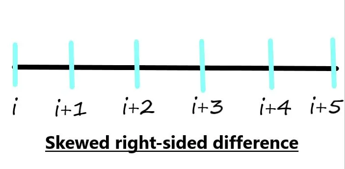
The distance between two nodes is `Deltax``

The 2nd order derivative for the 4th order approximation can be obtained by solving the following equation,

`f(u,x) => f'' ~= a*f(i)+b*f(i+1)+c*f(i+2)+d*f(i+3)+e*f(i+4)+g*f(i+5)``=>2`

It can be solved using taylor table,

Stensils`darr`\	f(i)	`Deltax*f'(i)`	`Deltax^2*f''(i)`	`Deltax^3*f'''(i)`	`Deltax^4*f''''(i)`	`Deltax^5*f'''''(i)`
a*f(i)	a	0	0	0	0	0
b*f(i+1)	b	b	b/2	b/6	b/24	b/120
c*f(i+2)	c	2c	`(4c)/2`	`(8c)/6`	`(16c)/24`	`(32c)/120`
d*f(i+3)	d	3d	`(9d)/2`	`(27d)/6`	`(81d)/24`	`(243d)/120`
e*f(i+4)	e	4e	`(16e)/2`	`(64e)/6`	`(256e)/24`	`(1024e)/120`
g*f(i+5)	g	5g	`(25g)/2`	`(125g)/6`	`(625g)/24`	`(3125g)/120`

By solving the taylor table based on eqn 2, 6 equations with 6 unknowns are obtained. Since the order of derivative is 2 all the other terms except `f''`is equalised to 0.

`a+b+c+d+e+g=0`

`0+b+2c+3d+4e+5g=0`

`0+b/2+(4c)/2+(9d)/2+(16e)/2+(25g)/2=1`

`0+b/6+(8c)/6+(27d)/6+(64e)/6+(125g)/6=0`

`0+b/24+(16c)/24+(81d)/24+(256e)/24+(625g)/24=0`

`0+b/120+(32c)/120+(243d)/120+(1024e)/120+(3125g)/120=0`

By solving the above equations, the values for the variables are obtained as

a=3.750000000000021,

b=-12.833333333333435,

c=17.833333333333520,

d=-13.000000000000170,

e=5.083333333333411 and

g=-0.833333333333348

By solving the equation 2 using taylor table,

`(a*f(i)+b*f(i+1)+c*f(i+2)+d*f(i+3)+e*f(i+4)+g*f(i+5))/(Deltax^2) = f''(i)`

By substituting the values for a,b,c,d,e and g,

`f''(i)=(3.750000000000021*f(i)-12.833333333333435*f(i+1)+17.833333333333520*f(i+2)-13.000000000000170*f(i+3)+5.083333333333411*f(i+4)-0.833333333333348*f(i+5))/(Deltax^2)`

The above equation is considered as the 4th order approximation of second order derivative using skewed right-sided difference scheme.

Skewed left-sided difference scheme:

The number of nodes can be calculated from the formula, n=p+q for skewed right-sided difference and skewed left-sided difference.

p = 2 (2nd order derivative)

q = 4 (4th order approximation)

n = p+q

= (2+4)

number of nodes = 6

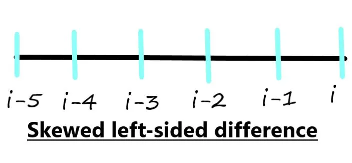
The distance between two nodes is `Deltax``

The 2nd order derivative for the 4th order approximation can be obtained by solving the following equation,

`f(u,x) => f'' ~= a*f(i)+b*f(i-1)+c*f(i-2)+d*f(i-3)+e*f(i-4)+g*f(i-5)``=>3`

It can be solved using taylor table,

Stensils`darr`\	f(i)	`Deltax*f'(i)`	`Deltax^2*f''(i)`	`Deltax^3*f'''(i)`	`Deltax^4*f''''(i)`	`Deltax^5*f'''''(i)`
a*f(i)	a	0	0	0	0	0
b*f(i-1)	b	-b	b/2	-b/6	b/24	-b/120
c*f(i-2)	c	-2c	`(4c)/2`	`-(8c)/6`	`(16c)/24`	`-(32c)/120`
d*f(i-3)	d	-3d	`(9d)/2`	`-(27d)/6`	`(81d)/24`	`-(243d)/120`
e*f(i-4)	e	-4e	`(16e)/2`	`-(64e)/6`	`(256e)/24`	`-(1024e)/120`
g*f(i-5)	g	-5g	`(25g)/2`	`-(125g)/6`	`(625g)/24`	`-(3125g)/120`

By solving the taylor table based on eqn 2, 6 equations with 6 unknowns are obtained. Since the order of derivative is 2 all the other terms except `f''`is equalised to 0.

`a+b+c+d+e+g=0`

`0-b-2c-3d-4e-5g=0`

`0+b/2+(4c)/2+(9d)/2+(16e)/2+(25g)/2=1`

`0-b/6-(8c)/6-(27d)/6-(64e)/6-(125g)/6=0`

`0+b/24+(16c)/24+(81d)/24+(256e)/24+(625g)/24=0`

`0-b/120-(32c)/120-(243d)/120-(1024e)/120-(3125g)/120=0`

By solving the above equations, the values for the variables are obtained as

a=3.750000000000021,

b=-12.833333333333435,

c=17.833333333333520,

d=-13.000000000000170,

e=5.083333333333411 and

g=-0.833333333333348

By solving the equation 2 using taylor table,

`(a*f(i)+b*f(i-1)+c*f(i-2)+d*f(i-3)+e*f(i-4)+g*f(i-5))/(Deltax^2) = f''(i)`

By substituting the values for a,b,c,d,e and g,

`f''(i)=(3.750000000000021*f(i)-12.833333333333435*f(i-1)+17.833333333333520*f(i-2)-13.000000000000170*f(i-3)+5.083333333333411*f(i-4)-0.833333333333348*f(i-5))/(Deltax^2)`

The above equation is considered as the 4th order approximation of second order derivative using skewed left-sided difference scheme.

Code:

The code to calculate the error of 4th order approximation of second order derivative using central difference scheme, skewed right-sided difference scheme and skewed left-sided difference scheme for the function exp(x)*cos(x) is shown below,

clear all
close all
clc

% Initializing x value and the function
x=pi/3;
fn = exp(x)*cos(x);

%dx value
dx = linspace(pi/3,pi/400,40);

% error calculation
for i=1:length(dx);
    error_cd(i) = central_difference(x,dx(i))
    error_SRD(i) = skewed_rightside_difference(x,dx(i))
    error_SLD(i) = skewed_leftside_difference(x,dx(i))
end


%plotting the errors
loglog(dx,error_cd,'-D','color','b')
hold on
loglog(dx,error_SRD,'-*','color','k')
hold on 
loglog(dx,error_SLD,'-o','color','r')
xlabel('dx')
ylabel('Errors')
title('Representation of errors (dx vs errors plot)')
legend('Central difference','Skewed right sided difference','Skewed left sided difference')

Function to calculate the error in central difference scheme,

function error_cd = central_difference(x,dx)

%Analytical value calculation
analytical = -2*exp(x)*sin(x);

%2nd order derivative with 4th order approximation
cd = ((-(0.083333333333334)*exp(x-dx-dx)*cos(x-dx-dx))+((1.333333333333334)*exp(x-dx)*cos(x-dx))-((2.500000000000001)*exp(x)*cos(x))+((1.333333333333334)*exp(x+dx)*cos(x+dx))-((0.083333333333334)*exp(x+dx+dx)*cos(x+dx+dx)))/dx^2;

%error calculations
error_cd = abs(cd-analytical);

end

Function to calculate the error in skewed right-sided difference scheme,

function error_SRD = skewed_rightside_difference(x,dx)

%Analytical value calculation
analytical = -2*exp(x)*sin(x);

%2nd order derivative with 4th order approximation
SRD = ((3.750000000000021*exp(x)*cos(x))-(12.833333333333435*exp(x+dx)*cos(x+dx))+(17.833333333333520*exp(x+dx+dx)*cos(x+dx+dx))-(13.000000000000170*exp(x+dx+dx+dx)*cos(x+dx+dx+dx))+(5.083333333333411*exp(x+dx+dx+dx+dx)*cos(x+dx+dx+dx+dx))-(0.833333333333348*exp(x+dx+dx+dx+dx+dx)*cos(x+dx+dx+dx+dx+dx)))/dx^2;

%error calculations
error_SRD = abs(SRD-analytical);
end

Function to calculate the error in skewed left-sided difference scheme,

function error_SLD = skewed_leftside_difference(x,dx)

%Analytical value calculation
analytical = -2*exp(x)*sin(x);

%2nd order derivative with 4th order approximation
SLD = ((3.750000000000021*exp(x)*cos(x))-(12.833333333333435*exp(x-dx)*cos(x-dx))+(17.833333333333520*exp(x-dx-dx)*cos(x-dx-dx))-(13.000000000000170*exp(x-dx-dx-dx)*cos(x-dx-dx-dx))+(5.083333333333411*exp(x-dx-dx-dx-dx)*cos(x-dx-dx-dx-dx))-(0.833333333333348*exp(x-dx-dx-dx-dx-dx)*cos(x-dx-dx-dx-dx-dx)))/dx^2;

%error calculations
error_SLD = abs(SLD-analytical);

end

Output plot:

Conclusion:

• The output error plot which includes central difference scheme, skewed right-sided difference scheme and skewed left-sided difference scheme clearly exhibit that the absolute error is minimum for the central difference scheme compared with other two schemes.
• The truncation error can be minimised by increasing the order of approximation.
• Skewed schemes play a vital role in many calculations. The flow can be easily analysed by providing the initial boundary condition in skewed schemes. The central difference scheme may also help, but there should be some consideration of imaginary nodes on the other side of the boundary condition.
• Also, it will be difficult to find the central reference node in many cases. So, skewed schemes provide the results by taking the successive nodes from the reference node.