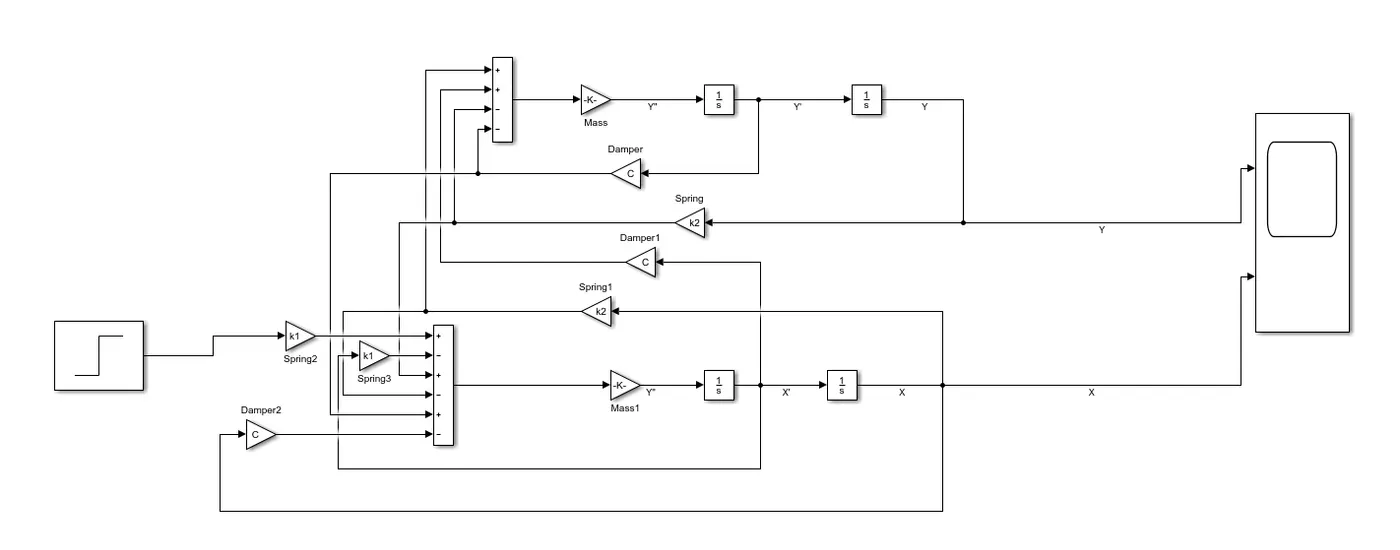
Suspension System of a car || MATLAB & Simulink

Suspension System Of a Car:

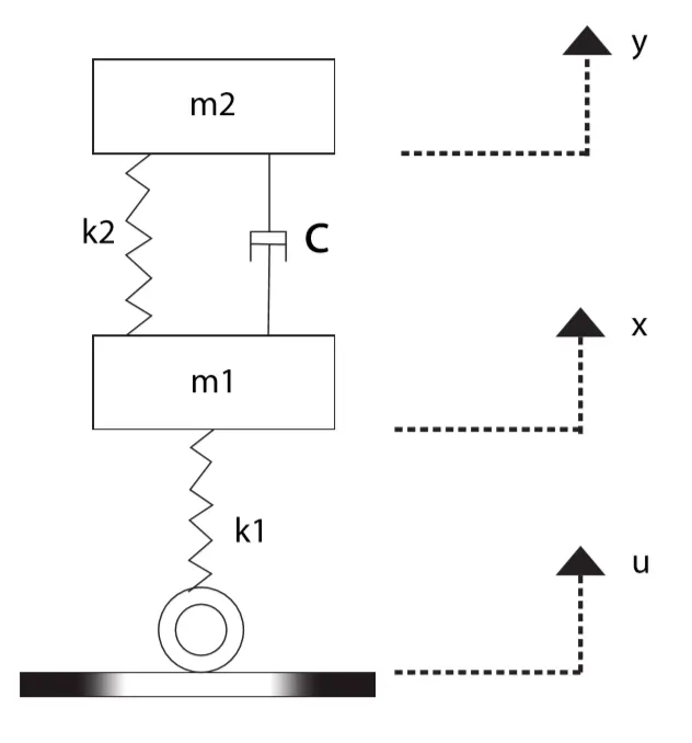
Diag.-1: Mass-Spring-Damper

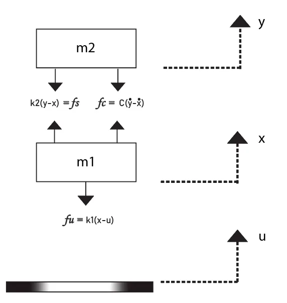
Diag.-2: Free Body Diagram

Here,

m2 = 14th">14th14th Mass of the car, Sprung Mass

m1 = Mass of the Wheel ,Unsprung Mass

K2,C = Suspension, Stiffness of the spring and Damper's Coefficient

K1 = Stiffness of the Tire

Let,

x=0, y=0 When System is in static equilibrium (allows gravity to be neglected)

Assume, Linear Springs and Damper, Negligible damping in the Tire.

From, Newton's 2nd law of motion,

we know that,

∑F=M⋅a">∑F=M⋅a∑F=M⋅a

For, mass m2

⇒">⇒⇒-fs-fc=m2⋅y..">−fs−fc=m2⋅..y-fs-fc=m2⋅y..

⇒">⇒⇒-k2(y-x)-c(y.-x.)=m2⋅y..">−k2(y−x)−c(.y−.x)=m2⋅..y-k2(y-x)-c(y.-x.)=m2⋅y..

⇒">⇒⇒m2⋅y..+c⋅y.+k2⋅y=c⋅x.+k2⋅x">m2⋅..y+c⋅.y+k2⋅y=c⋅.x+k2⋅xm2⋅y..+c⋅y.+k2⋅y=c⋅x.+k2⋅x Eqn 1">Eqn 1Eqn 1

Similarly,

For, mass m1

⇒">⇒⇒fs+fc-fu=m1⋅x..">fs+fc−fu=m1⋅..xfs+fc-fu=m1⋅x..

⇒">⇒⇒k2(y-x)+c(y.-x.)-k1(x-u)=m1⋅x..">k2(y−x)+c(.y−.x)−k1(x−u)=m1⋅..xk2(y-x)+c(y.-x.)-k1(x-u)=m1⋅x..

⇒m1⋅x..+c⋅x.+k1x+k2x=cy.+k2y+k1u">⇒m1⋅..x+c⋅.x+k1x+k2x=c.y+k2y+k1u⇒m1⋅x..+c⋅x.+k1x+k2x=cy.+k2y+k1uEqn 2">Eqn 2Eqn 2`

Writing, equation 1 and 2 in the form of time(t)

We have,

m2⋅y..(t)+c⋅y.(t)+k2⋅y(t)=c⋅x.(t)+k2⋅x(t)">m2⋅..y(t)+c⋅.y(t)+k2⋅y(t)=c⋅.x(t)+k2⋅x(t)m2⋅y..(t)+c⋅y.(t)+k2⋅y(t)=c⋅x.(t)+k2⋅x(t)

(a) Laplace tranform for this could be,

S2m2y(s)+Scy(s)+k2⋅y(s)=Scx(s)+k2⋅x(s)">S2m2y(s)+Scy(s)+k2⋅y(s)=Scx(s)+k2⋅x(s)S2m2y(s)+Scy(s)+k2⋅y(s)=Scx(s)+k2⋅x(s)

Rearranging,

x(s)=(S2m2+Sc+k2Sc+k2)⋅y(s)">x(s)=(S2m2+Sc+k2Sc+k2)⋅y(s)x(s)=(S2m2+Sc+k2Sc+k2)⋅y(s) Eqn 3">Eqn 3Eqn 3

Similarly,

For equation 2

we get,

x(s)(S2m1+Sc+k1+k2k1)-y(s)(Sc+k2k1)=u(s)">x(s)(S2m1+Sc+k1+k2k1)−y(s)(Sc+k2k1)=u(s)x(s)(S2m1+Sc+k1+k2k1)-y(s)(Sc+k2k1)=u(s) Eqn 4">Eqn 4Eqn 4

Now, Substituting the value of x(s)">x(s)x(s)from equation 3 in equation 4

We have,

⇒">⇒⇒outputinput=y(s)u(s)=Sk1c+k1k2S4m1m2+S3(m2c+m1c)+S2(m2k1+m2k2+c2+m1k2)+S(ck1)+k1k2">outputinput=y(s)u(s)=Sk1c+k1k2S4m1m2+S3(m2c+m1c)+S2(m2k1+m2k2+c2+m1k2)+S(ck1)+k1k2outputinput=y(s)u(s)=Sk1c+k1k2S4m1m2+S3(m2c+m1c)+S2(m2k1+m2k2+c2+m1k2)+S(ck1)+k1k2

(b) For State space function,

Let us, take equation 1 & 2, i.e.,

⇒m2⋅y..+c⋅y.+k2⋅y=c⋅x.+k2⋅x">⇒m2⋅..y+c⋅.y+k2⋅y=c⋅.x+k2⋅x⇒m2⋅y..+c⋅y.+k2⋅y=c⋅x.+k2⋅x Eqn 1">Eqn 1Eqn 1`

⇒m1⋅x..+c⋅x.+k1x+k2x=cy.+k2y+k1u">⇒m1⋅..x+c⋅.x+k1x+k2x=c.y+k2y+k1u⇒m1⋅x..+c⋅x.+k1x+k2x=cy.+k2y+k1uEqn 2">Eqn 2Eqn 2`

We Know the, standard state space equation

X.=AX+BU">.X=AX+BUX.=AX+BU

Y=CX+DU">Y=CX+DUY=CX+DU

So State Variables could be,

X1=y;X2=x;X3=y.=X.1;X4=x.=X.2;y..=X.3;x..=X.4">X1=y;X2=x;X3=.y=.X1;X4=.x=.X2;..y=.X3;..x=.X4X1=y;X2=x;X3=y.=X.1;X4=x.=X.2;y..=X.3;x..=X.4

Now, Substituting State Variables in Eqn 1 & 2, We get,

X.3=-k2m2⋅X1+k2m2⋅X2-cm2⋅X3+cm2⋅X4">.X3=−k2m2⋅X1+k2m2⋅X2−cm2⋅X3+cm2⋅X4X.3=-k2m2⋅X1+k2m2⋅X2-cm2⋅X3+cm2⋅X4

&

X.4=k2m1⋅X1-(k2+k1)m1m2⋅X2+cm1⋅X3-cm1⋅X4+k1m1⋅u">.X4=k2m1⋅X1−(k2+k1)m1m2⋅X2+cm1⋅X3−cm1⋅X4+k1m1⋅uX.4=k2m1⋅X1-(k2+k1)m1m2⋅X2+cm1⋅X3-cm1⋅X4+k1m1⋅u

So the Standard State Space Matrix should be,

[X.1X.2X.3X.4]=[00100001-k2m2k2m2-cm2cm2k2m1-(k1+k2m1m2)cm1-cm1][X1X2X3X4]+[000k1m1]⋅u">⎡⎢ ⎢ ⎢ ⎢ ⎢ ⎢⎣.X1.X2.X3.X4⎤⎥ ⎥ ⎥ ⎥ ⎥ ⎥⎦=⎡⎢ ⎢ ⎢ ⎢ ⎢ ⎢⎣00100001−k2m2k2m2−cm2cm2k2m1−(k1+k2m1m2)cm1−cm1⎤⎥ ⎥ ⎥ ⎥ ⎥ ⎥⎦⎡⎢ ⎢ ⎢ ⎢⎣X1X2X3X4⎤⎥ ⎥ ⎥ ⎥⎦+⎡⎢ ⎢ ⎢ ⎢ ⎢⎣000k1m1⎤⎥ ⎥ ⎥ ⎥ ⎥⎦⋅u[X.1X.2X.3X.4]=[00100001-k2m2k2m2-cm2cm2k2m1-(k1+k2m1m2)cm1-cm1][X1X2X3X4]+[000k1m1]⋅u

&

[yx]=[10000100]][X1X2X3X4]+(0)u">[yx]=[10000100]⎤⎥ ⎥ ⎥ ⎥⎦⎡⎢ ⎢ ⎢ ⎢⎣X1X2X3X4⎤⎥ ⎥ ⎥ ⎥⎦+(0)u[yx]=[10000100]][X1X2X3X4]+(0)u

3.

RC Circuit:

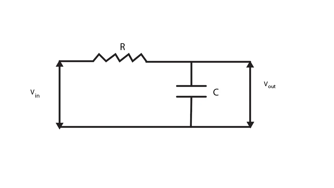
Applying KVL on this,

we get,

Vin=Ri(t)+1C∫i(t)dt">Vin=Ri(t)+1C∫i(t)dtVin=Ri(t)+1C∫i(t)dt-------(1)

Vout=1C∫i(t)dt">Vout=1C∫i(t)dtVout=1C∫i(t)dt------------(2)

Appliying Laplace on both Sides in Equation 1 & 2

we have,

Vin(s)=RI(S)+1CI(S)">Vin(s)=RI(S)+1CI(S)Vin(s)=RI(S)+1CI(S)

Vout(S)=1CI(S)">Vout(S)=1CI(S)Vout(S)=1CI(S)

Now,

Vout(S)Vin(S)=1CI(S)RI(S)+1CI(S)">Vout(S)Vin(S)=1CI(S)RI(S)+1CI(S)Vout(S)Vin(S)=1CI(S)RI(S)+1CI(S)

⇒Vout(S)Vin(S)=11+RC(S)">⇒Vout(S)Vin(S)=11+RC(S)⇒Vout(S)Vin(S)=11+RC(S)

CR Circuit:

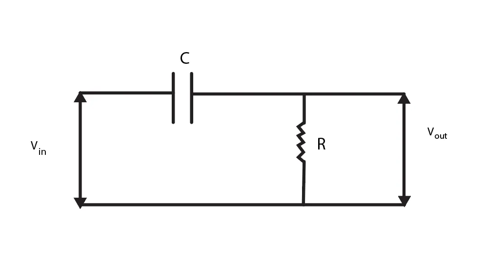
Applying KVL on this,

we get,

Vin=1C∫i(t)dt+Ri(t)">Vin=1C∫i(t)dt+Ri(t)Vin=1C∫i(t)dt+Ri(t)------------(1)

Vout=Ri(t)">Vout=Ri(t)Vout=Ri(t)t`------------(2)

Appliying Laplace on both Sides in Equation 1 & 2

we have,

Vin(S)=1CI(S)+RI(S)">Vin(S)=1CI(S)+RI(S)Vin(S)=1CI(S)+RI(S)

Vout(S)=RI(S)">Vout(S)=RI(S)Vout(S)=RI(S)

Now,

Vout(S)Vin(S)=RI(S)1CI(S)+IR(S)">Vout(S)Vin(S)=RI(S)1CI(S)+IR(S)Vout(S)Vin(S)=RI(S)1CI(S)+IR(S)

⇒Vout(S)Vin(S)=RC(S)1+CR(S)">⇒Vout(S)Vin(S)=RC(S)1+CR(S)

Mathematical Reprentation: