Supervised Learning - Prediction Week 3 Challenge

1.Perform Gradient Descent in Python with any loss function

Gradient Descent is an iterative algorithm that is used to minimize a function by finding the optimal parameters. Gradient Descent can be applied to any dimension function i.e. 1-D, 2-D, 3-D. In this article, we will be working on finding global minima for parabolic function (2-D) and will be implementing gradient descent in python to find the optimal parameters for the linear regression equation (1-D). Before diving into the implementation part, let us make sure the set of parameters required to implement the gradient descent algorithm. To implement a gradient descent algorithm, we require a cost function that needs to be minimized, the number of iterations, a learning rate to determine the step size at each iteration while moving towards the minimum, partial derivates for weight & bias to update the parameters at each iteration, and a prediction function.

Till now we have seen the parameters required for gradient descent. Now let us map the parameters with the gradient descent algorithm and work on an example to better understand gradient descent. Let us consider a parabolic equation y=4x². By looking at the equation we can identify that the parabolic function is minimum at x = 0 i.e. at x=0, y=0. Therefore x=0 is the local minima of the parabolic function y=4x². Now let us see the algorithm for gradient descent and how we can obtain the local minima by applying gradient descent:

Algorithm for Gradient Descent

Steps should be made in proportion to the negative of the function gradient (move away from the gradient) at the current point to find local minima. Gradient Ascent is the procedure for approaching a local maximum of a function by taking steps proportional to the positive of the gradient (moving towards the gradient).

repeat until convergence
{
    w = w - (learning_rate * (dJ/dw))
    b = b - (learning_rate * (dJ/db))
}

Calculate the loss = h - y and maybe the squared cost (loss^2)/2m. Calculate the gradient = X' * loss / m

In machine learning, gradients are used in gradient descent. We often have a loss function of many variables that we are trying to minimize, and we try to do this by following the negative of the gradient of the function. Note that a gradient is a vector, so it has both of the following characteristics: a direction.

2.Difference between L1 & L2 Gradient descent method.

L2 Loss function. Least absolute deviations(L1) and Least square errors(L2) are the two standard loss functions, that decides what function should be minimized while learning from a dataset. On the other hand, L2 loss function minimizes the squared differences between the estimated and existing target values.

L1 regularization penalizes the sum of absolute values of the weights, whereas L2 regularization penalizes the sum of squares of the weights.

3.What are the different loss functions for regression.

1. Mean Square Error, Quadratic loss, L2 Loss

Mean Square Error (MSE) is the most commonly used regression loss function. MSE is the sum of squared distances between our target variable and predicted values.

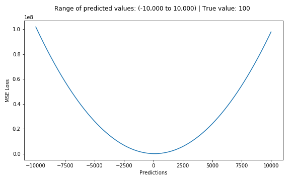
Below is a plot of an MSE function where the true target value is 100, and the predicted values range between -10,000 to 10,000. The MSE loss (Y-axis) reaches its minimum value at prediction (X-axis) = 100. The range is 0 to ∞.

2. Mean Absolute Error, L1 Loss

Mean Absolute Error (MAE) is another loss function used for regression models. MAE is the sum of absolute differences between our target and predicted variables. So it measures the average magnitude of errors in a set of predictions, without considering their directions. (If we consider directions also, that would be called Mean Bias Error (MBE), which is a sum of residuals/errors). The range is also 0 to ∞.

MSE vs. MAE (L2 loss vs L1 loss)

In short, using the squared error is easier to solve, but using the absolute error is more robust to outliers. But let’s understand why!

Whenever we train a machine learning model, our goal is to find the point that minimizes loss function. Of course, both functions reach the minimum when the prediction is exactly equal to the true value.

Here’s a quick review of python code for both. We can either write our own functions or use sklearn’s built-in metrics functions:

3. Huber Loss, Smooth Mean Absolute Error

Huber loss is less sensitive to outliers in data than the squared error loss. It’s also differentiable at 0. It’s basically absolute error, which becomes quadratic when error is small. How small that error has to be to make it quadratic depends on a hyperparameter, 𝛿 (delta), which can be tuned. Huber loss approaches MSE when 𝛿 ~ 0 and MAE when 𝛿 ~ ∞ (large numbers.)

The choice of delta is critical because it determines what you’re willing to consider as an outlier. Residuals larger than delta are minimized with L1 (which is less sensitive to large outliers), while residuals smaller than delta are minimized “appropriately” with L2.

Why use Huber Loss?
One big problem with using MAE for training of neural nets is its constantly large gradient, which can lead to missing minima at the end of training using gradient descent. For MSE, gradient decreases as the loss gets close to its minima, making it more precise.

Huber loss can be really helpful in such cases, as it curves around the minima which decreases the gradient. And it’s more robust to outliers than MSE. Therefore, it combines good properties from both MSE and MAE. However, the problem with Huber loss is that we might need to train hyperparameter delta which is an iterative process.

4. Log-Cosh Loss

Log-cosh is another function used in regression tasks that’s smoother than L2. Log-cosh is the logarithm of the hyperbolic cosine of the prediction error.

Advantage: log(cosh(x)) is approximately equal to (x ** 2) / 2 for small x and to abs(x) - log(2) for large x. This means that 'logcosh' works mostly like the mean squared error, but will not be so strongly affected by the occasional wildly incorrect prediction. It has all the advantages of Huber loss, and it’s twice differentiable everywhere, unlike Huber loss.

4.What is the importance of learning rate.

The learning rate controls how quickly the model is adapted to the problem. Smaller learning rates require more training epochs given the smaller changes made to the weights each update, whereas larger learning rates result in rapid changes and require fewer training epochs

This parameter determines how fast or slow we will move towards the optimal weights. If the learning rate is very large we will skip the optimal solution. If it is too small we will need too many iterations to converge to the best values. So using a good learning rate is crucial.

5.How to evaluate linear regression.

R Square/Adjusted R Square : This is a first measure of regression model especially we, everybody, do during evaluation because it is easy to interpret score between 0 to 1. If we see good score like close to 1, then we assume that model is good fit

Mathematically, the RMSE is the square root of the mean squared error (MSE), which is the average squared difference between the observed actual outome values and the values predicted by the model. So, MSE = mean((observeds - predicteds)^2) and RMSE = sqrt(MSE ). The lower the RMSE, the better the model.

Mean absolute error (MAE) is a loss function used for regression. Use MAE when you are doing regression and don't want outliers to play a big role. The loss is the mean over the absolute differences between true and predicted values, deviations in either direction from the true value are treated the same way.

6.What is the difference between multiple and adjusted coefficient of determination

The fundamental point is that when you add predictors to your model, the multiple Rsquared will always increase, as a predictor will always explain some portion of the variance. Adjusted Rsquared controls against this increase, and adds penalties for the number of predictors in the model.

Clearly, it is better to use Adjusted R-squared when there are multiple variables in the regression model. This would allow us to compare models with differing numbers of independent variables

What is the Adjusted Coefficient of Determination? The Adjusted Coefficient of Determination (Adjusted R-squared) is an adjustment for the Coefficient of Determination that takes into account the number of variables in a data set. It also penalizes you for points that don't fit the model.